Applying the Monte Carlo method for optimizing trading strategies

Contents

• General theory
• Probabilistic EA model
• Applying the theory
• Profit robustness against random scatter
• Profit robustness against drawdown
• Profit distribution robustness against price nonstationarity
• Conclusion
• Attached files
  

General theory

The idea beyond Monte Carlo method can be described in terms of analogy — one of scientific knowledge methods. Other examples of analogy are Hamilton's optico-mechanical analogy or similar organs in biology.

If we have two objects that can be described by the same theory, then the knowledge gained from studying one of them is applicable to another. This method is very useful when one object is much easier to study than the other. The more accessible object is considered a model of another one. The method itself is called modeling. Depending on a context, a model is one of the objects or a theory common for both of them.

Sometimes, researchers misunderstand modeling results. When we consider some explicit examples, like blowing off a reduced copy of an airplane in a wind tunnel, everything seems obvious. However, when objects are not related and do not look alike at first sight, the conclusions sometimes seem to be some kind of a trick or serve as a basis for unreasonable but far-reaching generalizations. Common theory for objects roughly describes only some of their aspects. The less the required accuracy of objects description, the wider the set of objects that adhere to a theory. For example, Hamilton's optico-mechanical analogy is exactly satisfied only when the length of a light wave tends to zero. In reality, this analogy is approximately justified only for a small but always finite length. Since any theoretical model should be simple enough to serve as a basis for calculations and conclusions, it is always oversimplified.

Let's now clarify the concept of the Monte Carlo method. This is an approach to modeling objects whose theory has a probabilistic (stochastic) nature. The model is a computer program with an algorithm constructed in accordance with this theory. It uses pseudo-random number generators to simulate the necessary random variables (random processes) with the required distributions.

It is worth emphasizing (although it does not matter for us here) that the nature of a studied object can be both probabilistic and deterministic. The presence of a theory having a probabilistic nature is of importance for us here. For example, Monte Carlo method is used to approximately calculate ordinary integrals. This is possible, because any such integral can be regarded as a mathematical expectation of a random variable.

The first example of using Monte Carlo method is usually considered to be a solution of the Buffon's needle problem in which the Pi number is determined by randomly throwing a needle on a table. The name of the method appeared much later, in the middle of the XX century. After all, gambling games — for example, a roulette — are random number generators. Besides, a deliberate reference to gambling hints at the origins of probability theory, which began with calculations related to playing dice and cards.

The modeling program algorithm is simple, which is one of the reasons for the method prevalence. The algorithm features multiple randomly generated variants (samples) of a studied object state with the distribution corresponding to the theory. A required set of characteristics is calculated for each of them. As a result, we receive a large sample. While we have only one set of characteristics for the studied object, the Monte Carlo method allows us to get them in large numbers and construct their distribution functions, which gives us more data.

The general Monte Carlo modeling structure described above seems simple. However, it produces multiple and sometimes rather complex variations when trying to implement it. Even if we confine our application to finance, we still can see how extensive it is, for example in this book. We will try to apply the Monte Carlo method to study the stability of Expert Advisors. To achieve this, we need a probabilistic model describing their work.

Probabilistic EA model

Before starting a real trading using an EA, we usually test and optimize it in quotes history. But why do we believe that trading results in the past affect their results in the future? Naturally, we do not expect that all transactions in the future form the same sequence as in the past. Although we still have have an assumption about their "similarity". Let's formalize this intuitive idea of ​​"similarity" using the theory of probability. In accordance with this formalization, we believe that the result of each trade is a certain realization of some random variable. The "similarity" of trades in this case is determined through the proximity of the corresponding distribution functions. In such formalization, past trades help clarify the type of distribution for future ones and assess their possible outcomes.

Probabilistic formalization allows us to construct various theories. Let's consider the simplest and the most commonly used one. In this theory, a result of each trade is unambiguously defined by a relative profit k=C1/C0, where C0 and C1 are capital volumes before and after the trade. Further on, the relative trade profit will simply be called a profit, while the difference C1-C0 is an absolute trade profit. Suppose that profits of all trades (both in the past and in the future) are independent of each other and comprise of evenly distributed random values. Their distribution is determined by the F(x) distribution function. Thus, our task is to define the type of this function by using values of the past profitable trades. This is the standard problem of mathematical statistics — restoration of the distribution function by sample. Any of its solutions always provide approximate answers. Let's have a look at some of these methods.

1. Empirical distribution function is used as an approximation.

2. We take a simple discrete distribution, in which a trade profit takes one of the two values. This is either an average loss with a loss probability, or an average profit with a profit probability.

3. We construct not a discrete, but a continuous (having a density) approximation for the distribution function. To achieve this, we use such methods as kernel density estimation.
   

Further on, we will use the first option - it is the most simple and universal. Traders are not very interested in knowing the function itself. However, it is important to know what amounts indicate a possible profit from the EA operation, a risk level of its use or sustainability of profits. These values can be obtained knowing the distribution function.

Let's specify the modeling algorithm in our case. The object of our interest is a possible result of the EA operation in the future. It is unambiguously defined by the sequence of trades. Each trade is set by the profit value. The profits are distributed according to the empirical distribution described above. We should generate a large number of such sequences and calculate the necessary characteristics for each of them. The generation of each such sequence is simple. Let's define the sequence of trade profits obtained on history as k1, k2, ..., kn. By generating the sequences with the length of N, we will randomly (with the equal probability of 1/n) select one of ki (sample with return) N times. It is usually assumed that N=n, since at large N, the F(x) approximation accuracy by empirical distribution deteriorates. This version of Monte Carlo method is sometimes called the bootstrap method.

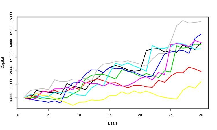
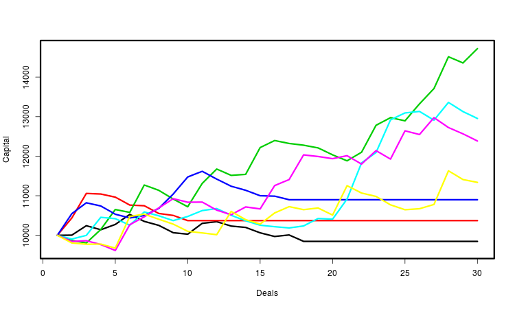
Let's explain all above by the graph. It shows several capital curves. Each of them is determined by the generated sequence of trades. I marked the curves with different colors for more convenience. In fact, their number is much larger — several tens of thousands. For each of them, we calculate the necessary parameters and make statistical conclusions based on their totality. Obviously, the most important of these characteristics is the final profit.

Other approaches to probabilistic formalization and further EA operation modeling are possible as well. For example, instead of sequences of trades, we can simulate price sequences and study the aggregate profits the EA has obtained on them. The principle of generating price series can be selected depending on a task you want to solve. However, this method requires much more computing resources. In addition, MetaTrader currently provides no regular ways to use it with a random EA.

Applying the theory

Our task is to construct specific optimization criteria. Each of them corresponds to a certain goal. The main one is the final profit obtained as a result of the whole series of trades. Optimization by profit is built into the tester. Since we are interested in profit in the future, we should somehow evaluate the possible degree of its deviation from profits in the present. The smaller the deviation, the more stable the profit of the system. Let's consider three approaches.

1. Having obtained a large sample of possible values ​​of profit through Monte Carlo method, we can study its distribution and the quantities associated with it. The average value of this profit is very important. The variance is also important — the smaller it is, the more stable the work of the EA and the less uncertainty in its future results. Our criterion will be equal to the ratio of the average profit to its average scatter. It is similar to the Sharpe ratio.
2. Another important characteristic is a drawdown of profits in a series of trades. Too much drawdown can lead to a loss of a deposit, even if the EA is profitable. For this reason, a drawdown is usually restricted. It is useful to know how it affects the possible profit. The criterion is defined simply as the average profit, but with the condition that the termination of trade is modeled when the allowable level of drawdown is exceeded.

3. We will construct a criterion measuring the stability of profit in terms of the persistence of the trade profits distribution. From the point of the probability theory, this means stationarity of trade profits, which, in principle, is possible in the case of non-stationary price increments. To do this, we will use an idea similar to forward testing. Let's divide the initial sample of trades into the initial and final subsamples. To verify their homogeneity, we can apply a statistical test. Based on this test, we will create an optimization criterion.
   

To demonstrate our theory, we will use the "Moving Average.mq5" EA included in the MetaTrader 5 delivery. We will implement small changes to its code. At the beginning of the EA, add a code string to include our header file:

#include <mcarlo.mqh>

Add the code for obtaining and using our optimization parameter at the end of the EA:

double OnTester()
  {
   return optpr();         // optimization parameter
  }

Basic calculations are made on functions located in the "mcarlo.mqh" header file. We place it to the "MQL5/Include/" folder. The main function in this file is optpr(). When the necessary conditions are met, it calculates the optimization criterion variant specified by the noptpr parameter, otherwise it returns zero.

double optpr()
  {
   if(noptpr<1||noptpr>NOPTPRMAX) return 0.0;
   double k[];
   if(!setks(k)) return 0.0;
   if(ArraySize(k)<NDEALSMIN) return 0.0;
   MathSrand(GetTickCount());
   switch(noptpr)
     {
      case 1: return mean_sd(k);
      case 2: return med_intq(k);
      case 3: return rmnd_abs(k);
      case 4: return rmnd_rel(k);
      case 5: return frw_wmw(k);
      case 6: return frw_wmw_prf(k);
     }
   return 0.0;
  }

The setks() function calculates the array of trade profits based on trading history.

bool setks(double &k[])
  {
   if(!HistorySelect(0,TimeCurrent())) return false;
   uint nhd=HistoryDealsTotal();
   int nk=0;
   ulong hdticket;
   double capital=TesterStatistics(STAT_INITIAL_DEPOSIT);
   long hdtype;
   double hdcommission,hdswap,hdprofit,hdprofit_full;
   for(uint n=0;n<nhd;++n)
     {
      hdticket=HistoryDealGetTicket(n);
      if(hdticket==0) continue;

      if(!HistoryDealGetInteger(hdticket,DEAL_TYPE,hdtype)) return false;
      if(hdtype!=DEAL_TYPE_BUY && hdtype!=DEAL_TYPE_SELL) continue;

      hdcommission=HistoryDealGetDouble(hdticket,DEAL_COMMISSION);
      hdswap=HistoryDealGetDouble(hdticket,DEAL_SWAP);
      hdprofit=HistoryDealGetDouble(hdticket,DEAL_PROFIT);
      if(hdcommission==0.0 && hdswap==0.0 && hdprofit==0.0) continue;

      ++nk;
      ArrayResize(k,nk,NADD);
      hdprofit_full=hdcommission+hdswap+hdprofit;
      k[nk-1]=1.0+hdprofit_full/capital;
      capital+=hdprofit_full;
     }
   return true;
  }

The sample() function generates a random b[] sequence from the original a[] sequence.

void sample(double &a[],double &b[])
  {
   int ner;
   double dnc;
   int na=ArraySize(a);
   for(int i=0; i<na;++i)
     {
      dnc=MathRandomUniform(0,na,ner);
      if(!MathIsValidNumber(dnc)) {Print("MathIsValidNumber(dnc) error ",ner); ExpertRemove();}
      int nc=(int)dnc;
      if(nc==na) nc=na-1;
      b[i]=a[nc];
     }
  }

Next, we will consider in detail each of the three types of optimization criteria mentioned above. In all cases, we will perform optimization on the same time interval - spring/summer 2017 for EURUSD. The timeframe will always be 1 hour, and the test mode is OHLC from a minute chart. The genetic algorithm by the custom optimization criterion will always be used. Since our task is to demonstrate the theory rather than preparing the EA for real trading, such simplistic approach seems natural.

Profit robustness against random scatter

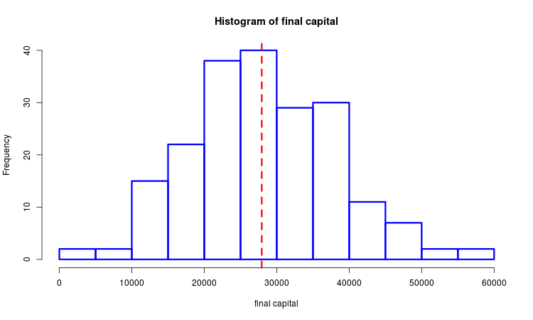
Suppose that we have a sample of generated final profits. We can study it with the help of mathematical statistics methods. The image below shows a histogram with a selected median marked with a dotted line.

We construct two similar versions of the optimization criterion. They are calculated in the mean_sd() and med_intq() functions. The common part of these options is that they represent the ratio of the mean to the measure of scatter. The difference is in how the average and the scatter measure are determined. In the first case, these are the arithmetic average and standard deviation, while in the second — selective median and interquartile range. The higher the profit and the lesser its scatter, the higher the values of both of them. There is an obvious similarity to the Sharpe ratio, although here we mean a profit in the entire series of trades rather than in a single trade. The second variant of the criterion is more resistant to spikes in comparison with the first one.

double mean_sd(double &k[])
  {
   double km[],cn[NSAMPLES];
   int nk=ArraySize(k);
   ArrayResize(km,nk);
   for(int n=0; n<NSAMPLES;++n)
     {
      sample(k,km);
      cn[n]=1.0;
      for(int i=0; i<nk;++i) cn[n]*=km[i];
      cn[n]-=1.0;
     }
   return MathMean(cn)/MathStandardDeviation(cn);
  }

double med_intq(double &k[])
  {
   double km[],cn[NSAMPLES];
   int nk=ArraySize(k);
   ArrayResize(km,nk);
   for(int n=0; n<NSAMPLES;++n)
     {
      sample(k,km);
      cn[n]=1.0;
      for(int i=0; i<nk;++i) cn[n]*=km[i];
      cn[n]-=1.0;
     }
   ArraySort(cn);
   return cn[(int)(0.5*NSAMPLES)]/(cn[(int)(0.75*NSAMPLES)]-cn[(int)(0.25*NSAMPLES)]);
  }

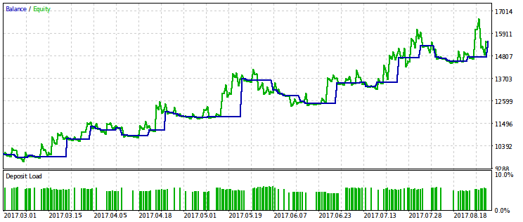
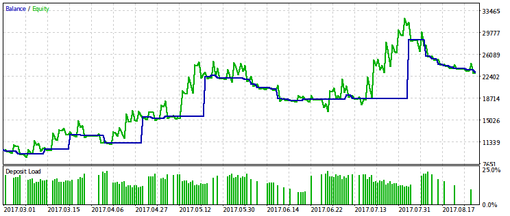
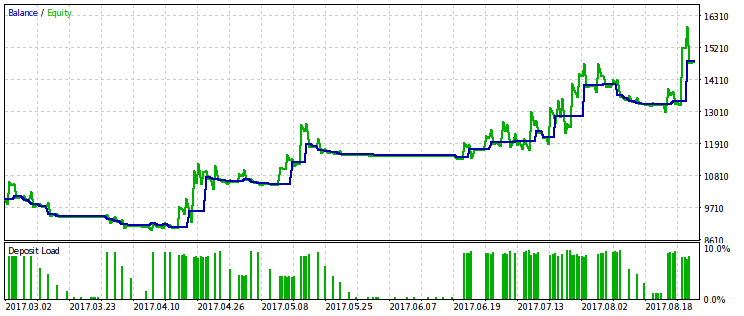
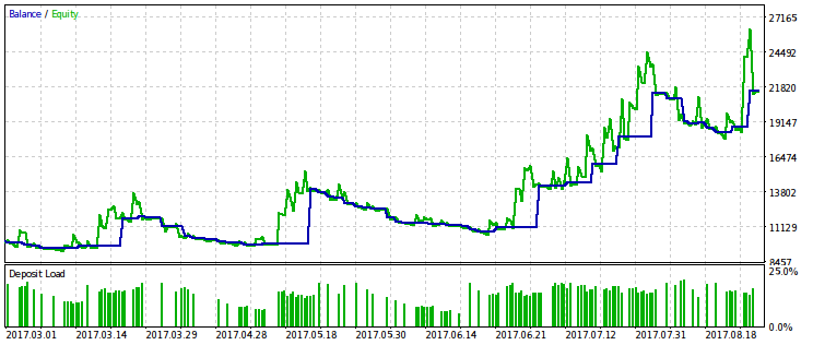
Below are two pairs of test results for the EA optimized by this criterion. On the first pair, there is an optimization result for the first variant and, for comparison, the result with the maximum profit. Obviously, the first one is preferable, since it gives a smoother capital curve. The final profit, if desired, can be increased by increasing the volume of trades.

The same pair of results is provided for the second variant of the optimization criterion. It is possible to draw the same conclusions from them.

Profit robustness against drawdown

We monitor the amount of drawdown in each generated sequence of trades. If the capital remaining after the initial part of the trade series comprises a smaller proportion than set by the rmndmin parameter, the remaining trades are discarded. The image below shows that the capital stops changing and the final section of the capital line becomes horizontal in case a relative drawdown level is exceeded.

We have two criterion calculation options — for absolute and relative drawdown. In case of an absolute drawdown, the share of the capital is calculated from its initial value, while in case of a relative drawdown, the calculation is done from the maximum one. The functions calculating these parameter variants are called rmnd_abs() and rmnd_rel() accordingly. In both cases, the value of the criterion is the average of the generated profits.

double rmnd_abs(double &k[])
  {
   if (rmndmin<=0.0||rmndmin>=1.0) return 0.0;
   double km[],cn[NSAMPLES];
   int nk=ArraySize(k);
   ArrayResize(km,nk);
   for(int n=0; n<NSAMPLES;++n)
     {
      sample(k,km);
      cn[n]=1.0;
      for(int i=0; i<nk;++i)
        {
         cn[n]*=km[i];
         if(cn[n]<rmndmin) break;
        }
      cn[n]-=1.0;
     }
   return MathMean(cn);
  }

double rmnd_rel(double &k[])
  {
   if (rmndmin<=0.0||rmndmin>=1.0) return 0.0;
   double km[],cn[NSAMPLES],x;
   int nk=ArraySize(k);
   ArrayResize(km,nk);
   for(int n=0; n<NSAMPLES;++n)
     {
      sample(k,km);
      x=cn[n]=1.0;
      for(int i=0; i<nk;++i)
        {
         cn[n]*=km[i];
         if(cn[n]>x) x=cn[n];
         else if(cn[n]/x<rmndmin) break;
        }
      cn[n]-=1.0;
     }
   return MathMean(cn);
  }

We can perform optimization either with a suitable rmndmin fixed parameter or to look for its optimal value.

Let's provide the results only for the criterion associated with the relative drawdown because its limitation gives a more pronounced effect. We will carry out optimization with several variants of the rmndmin fixed value: 0.95, 0.75 and 0.2.

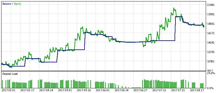
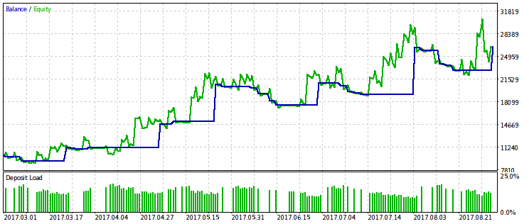
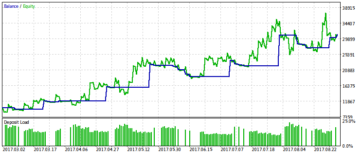
The lower the rmndmin value, the less noticeable the drawdown, while the results of optimization are more and more similar to those with the usual profit maximization. This can be considered a consequence of the law of large numbers – the probability theory principle. On the images, this effect is not immediately noticeable, because they have a different scale by the vertical axis (due to the adjustment of all images to the same dimensions). Besides, the increasing drawdown due to decreasing rmndmin value is not immediately apparent.

Now, let's include the rmndmin parameter to the number of optimized ones, and we will continue optimization by the same criterion.

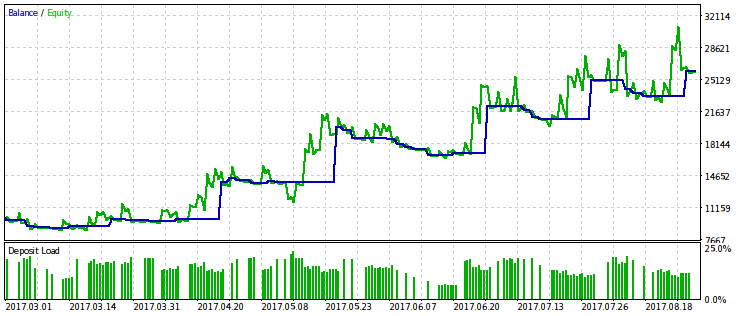
Get the optimal value rmndmin=0.55. With such a value, a drawdown may reach almost half of the account, which is unacceptable. Therefore, it is hardly usable in real trading. However, there is another benefit here. We can see that "waiting out" even greater drawdowns, most likely, does not make any sense. This corresponds to the second half of the trading rule: "Let your profit grow, cut off losses".

Profit distribution robustness against price nonstationarity

Price behavior may change. At the same time, we would like the results of the EA's work to be stable. From the point of our EA probability model, this means we need trade profit stationarity even in case of non-stationary price increments.

Our optimization criterion compares the initial part of the trade sequence with the final one. The closer they are, the greater its value. Closeness is determined based on the Wilcoxon-Mann-Whitney criterion. Let's explain its essence. Suppose that we have two samples of trades. The criterion determines how much one of the samples is shifted relative to another. The smaller the shift, the higher the criterion value. Let's explain this by the image. Each sample is represented by the corresponding histogram. The greatest value of the criterion can be found on the middle image.

In this case, Monte Carlo method itself is not used. However, the large value of the WMW criterion justifies its application, since it confirms the assumption that the type of trade profit distribution is preserved.

Our file also features another criterion variant — the product of WMW criterion by profit.

double frw_wmw(double &k[])
  {
   if (fwdsh<=0.0||fwdsh>=1.0) return 0.0;
   int nk=ArraySize(k), nkf=(int)(fwdsh*nk), nkp=nk-nkf;
   if(nkf<NDEALSMIN||nkp<NDEALSMIN) return 0.0;
   double u=0.0;
   for (int i=0; i<nkp; ++i)
     for (int j=0; j<nkf; ++j)
       if(k[i]>k[nkp+j]) ++u;
   return 1.0-MathAbs(1.0-2.0*u/(nkf*nkp));
  }

double frw_wmw_prf(double &k[])
  {
   int nk=ArraySize(k);
   double prf=1.0;
   for(int n=0; n<nk; ++n) prf*=k[n];
   prf-=1.0;
   if(prf>0.0) prf*=frw_wmw(k);
   return prf;
  }

Direct use of the WMW criterion is problematic since it can mistake a loss-making option for the optimal one. It would be better to optimize the EA by profit and discard options with a small value of this parameter, but it is still unclear how to do this. We can choose a number of the best options from the WMW criterion point of view, and then choose among them the one that gives a maximum profit.

We will provide examples of the two out of ten best passes. One of them is profitable, while another one is loss-making.

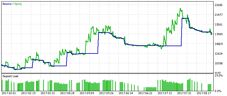
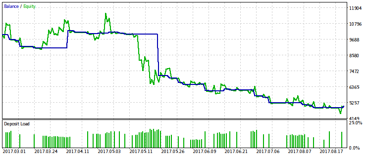
It seems that the WMW criterion would be more useful when comparing two different EAs on the same time interval or one EA on different time intervals. But it is not yet clear how to make such a comparison regular.

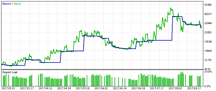
We will also give an example of optimization by a criterion equal to the product of the WMW-criterion by profit. Apparently, it is very similar to a simple optimization by profit, which means its use is excessive.

Conclusion

In this article, we have briefly touched some aspects of the marked topic. Let's conclude it with short remarks.

• The optimization criteria constructed in the article may help formalize intuitive ideas about the most efficient sequence of trades. This is useful when choosing from a large number of options.
  
• There are known measures for risk, like VaR (Value At Risk) or the ruin probability. If you use them directly as an optimization criterion, the result will be poor. Trading volumes and number of trades will be understated. Therefore, a compromise criterion is needed, which depends on the both variables — risk and profit. The question is, which version of this criterion we should choose, since the functions of the two variables are infinite. For example, the criterion may be selected based on the level of a trading strategy "aggressiveness", which varies greatly.
  
• Different variants of optimization criteria measuring stability can be useful for different EA classes. For instance, trend-following EAs will differ from the ones trading in a range, while systems featuring a fixed take profit will differ from the ones closing trades by a trailing stop. Profit distributions of such EAs will also belong to different classes. Depending on this, one or another criterion will be more appropriate.
• Some criteria are useful for comparing two different EAs rather than for comparing the behavior of the same EA on a fixed time interval at different sets of parameters. With the help of such criteria, it is possible to compare the work of a single EA at different time intervals.
  
• Monte Carlo modeling would be more complete if it were possible to pass not only the existing price history, but also its randomly altered copies to the EA's input. This would allow us to study the stability of EAs more thoroughly, albeit at the cost of increasing the amount of calculations.
  

Attached files

#	Name	Type	Description
1	Moving Average_mcarlo.mq5	Script	Modified standard Moving Average.mq5
2	mcarlo.mqh	Header file	Main file with the functions performing all necessary calculations