
Deep Neural Networks (Part III). Sample selection and dimensionality reduction
Contents
- Introduction
- 1. Sample selection
- 2. Dimensionality reduction
- 2.1. Principal component analysis (PCA)
- 2.2. Independent component analysis (ICA)
- 2.3. Probabilistic principal component analysis (PPCA)
- 2.4. Autoencoder (nonlinear PCA)
- 2.5. Inverse nonlinear PCA (NLPCA)
- 3. Dividing the data set into the train/valid/test sets
- Conclusion
- Application
Introduction
This is the third (and last) article describing data preparation - the most important stage of work with neural networks. We will consider two very important methods of preparing data. They are removing noise and reducing input dimensionality. Method descriptions will be accompanied by detailed examples and charts.
1. Sample selection
Noise samples refer to the wrong labeling of training samples. This is a very undesirable peculiarity of data. To overcome this we will use the NoiseFilterR package where classical and contemporary noise filters are R implemented.
Lately, data mining has had to deal with increasingly complex problems connected with the character of data. It is not the volume of the data but their imperfection and different forms present the explorers with a multitude of various scenarios. Consequently, preliminary data processing has become an important part of the KDD process (Knowledge Discovery from Databases). At the same time, the development of the software for preliminary data processing provides sufficient tools for work.
Preliminary data processing is required for the following algorithms to be able to extract maximum information from a data set. This is one of the most energy and time consuming stages in the whole process of KDD. Preliminary data processing can be divided into sub-tasks. For instance, these can be the selection of predictors or removing missing and noise data. The selection of predictors aims to extract the most important attributes for training, which allows to simplify models and reduce the calculation time. Processing of the missing data is necessary for storing as much data as possible. Noise data is either incorrect data or data that stand out from the data distribution.
All these problems can be solved with widely available software. For instance, the KEEL (RKEEL) tool contains a wide set of algorithms of preliminary data processing which covers all the manipulations mentioned above. There are other popular solutions like WEKA (RWEKA) or RapidMiner for selecting predictors. There is also a number of unique program complexes for Data Mining such as R, KNIME or Python.
As for the statistical software R, The Comprehensive R Archive Network (CRAN) contains a lot of packages for solving problems of preliminary data processing.
Real data sets always contain imperfections and noise. This noise has a negative impact on the training of classifiers, which in turn reduces prediction accuracy, overcomplicates models and increases calculation time.
Designated literature on classification distinguishes two different types of noise: the attribute noise and the labeling noise (or class noise). The first one occurs due to imperfections of the training data set attributes and the second one occurs because of the errors in the classification methods. The NoiseFiltersR package mainly focuses on the labeling noise - the most detrimental one as the quality of labeling is very important for training classifiers.
Two main approaches to solving the problem of labeling noise are described here. You can study them in detail in recent work by Benoit Frenay and Michel Verleysen.
- On the one hand, this is an approach at the algorithm level when a problem is solved by creating a robust classification algorithm which is not affected much by the presence of noise. Each algorithm in this case will be a specific, nonuniversal solution.
- On the other hand, an approach at the data level (filters) is an attempt to develop a strategy of cleaning data which will be carried out before the training of the classifier. The NoiseFiltersR package utilizes the second approach. This is because it allows preliminary data processing only once and after that classifiers can be changed as many times as required.
The following classifiers are resistant to noise: С4.5, J48 and Jrip (WEKA).
Let us conduct an experiment. Let us treat the following data sets: DT (raw data before preliminary processing), DTn (only normalized raw data set), DTTanh.n (without outliers, tan-transformed and normalized) and the train set with the ORBoostFilter() function, which is a filter for removing noise. Let us see how the distribution changed after such processing.
evalq({
  #-----DT---------------------
  out11 <- ORBoostFilter(Class~., data = DT$train, N = 10, useDecisionStump = TRUE)
  DT$train_clean1 <- out11$cleanData
  #----------DTTanh.n------------------------
  out1 <- ORBoostFilter(Class~., data = DTTanh.n$train, N = 10, useDecisionStump = TRUE)
  DTTanh.n$train_clean1 <- out1$cleanData
  #-----------DTn--------------------------------
  out12 <- ORBoostFilter(Class~., data = DTn$train, N = 10, useDecisionStump = TRUE)
  DTn$train_clean1 <- out12$cleanData
},
env)
#---Ris1-----------------
require(funModeling)
evalq({
  par(mfrow = c(1,3))
  par(las = 1)
  boxplot(DT$train_clean1 %>% select(-c(Data,Class)), horizontal = TRUE,
          main = "DT$train_clean1")
  boxplot(DTn$train_clean1 %>% select(-c(Data,Class)), horizontal = TRUE,
          main = "DTn$train_clean1")
  boxplot(DTTanh.n$train_clean1 %>% select(-c(Data,Class)), horizontal = TRUE,
          main = "DTTanh.n$train_clean1")
  par(mfrow = c(1,1))
}, env)
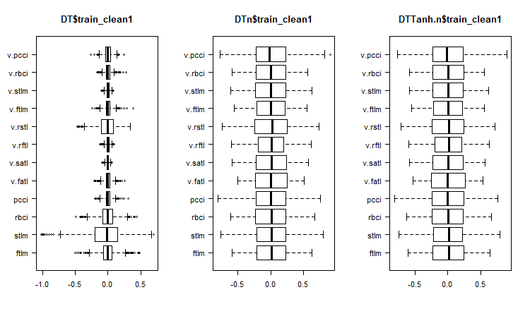
Fig. 1. Distribution of predictors in the sets after removing noise samples
Let us see what variation and covariance in these sets are:
#----Ris2------------------
require(GGally)
evalq(ggpairs(DT$train_clean1 %>% select(-Data),
              columns = c(1:6, 13),
              mapping = aes(color = Class),
              title = "DT$train_clean1/1"),
      env)
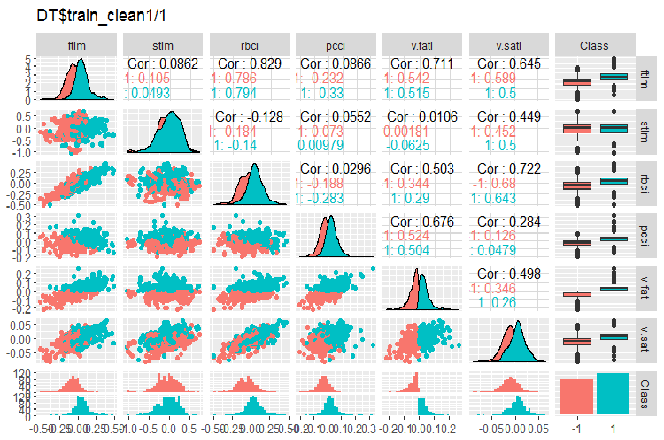
Fig. 2. Variation and covariance in the DT$train_clean1/1 set after removing noise samples
#-----Ris3---
evalq(ggpairs(DT$train_clean1 %>% select(-Data),
              columns = 7:13,
              mapping = aes(color = Class),
              title = "DT$train_clean1/2"),
      env)
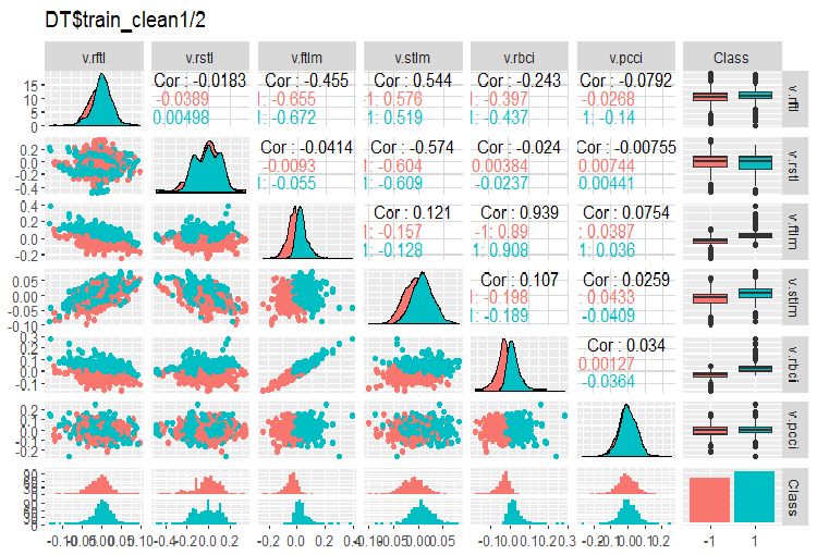
Fig. 3. Variation and covariance in the DT$train_clean1/2 set after removing noise samples
How many samples were removed from the DT$train set?
> env$out11$remIdx %>% length()
[1] 658
This is around 30%. There are two ways to go about it. The first one is to remove noise samples from the train set and pass it to the model for training. The second one is to rearrange them with a new class label and train the model on the full train set but with one additional level of the goal variable. With this number of noise samples, second scenario looks more favorable. We should test this.
What can we see on the charts of variable distributions without noise?
- Very distinctive division of the distribution of predictors by the goal variable. It is highly likely that this will significantly increase the accuracy of the model we are training.
- Nearly all outliers have been removed.
We are going to clean the DTn$train DTTanh.n$train data sets using the filter. You will be surprised to see that there are as many noise variables as there are in the first case.
c(env$out1$remIdx %>% length(), env$out12$remIdx %>% length())
[1] 652 653
Does this mean that no transformations make noise samples useful? This is worth testing.
Let us take a look at the variation and covariance of the DTTanh.n$train set after removing noise variables.
#----Ris4-----------------------
evalq(ggpairs(DTTanh.n$train_clean1, columns = 1:13,
              mapping = aes(color = Class),
              upper = "blank",
              title = "DTTanh.n$train_clean_all"),
      env)
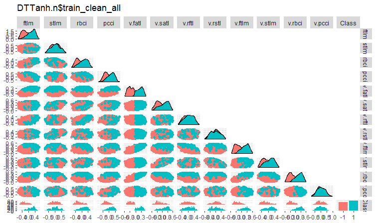
Fig. 4. Variation and covariance in the DTTanh.n$train_clean set after removing noise samples.
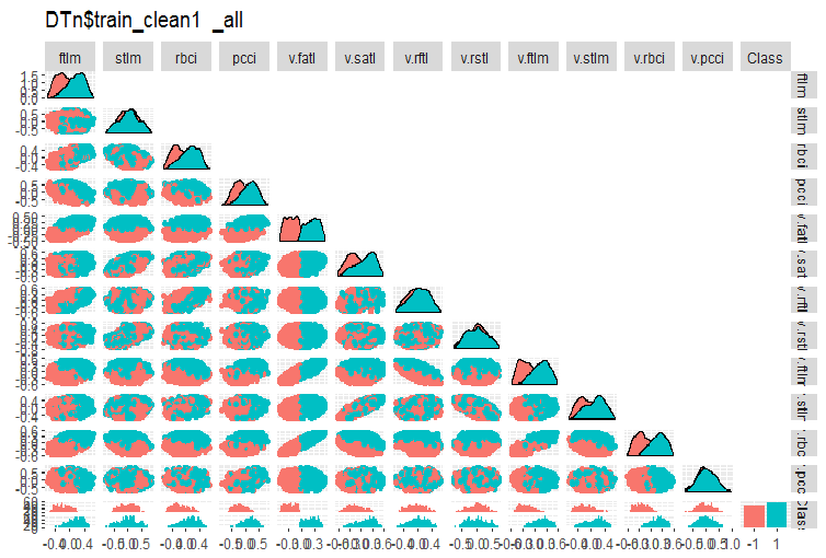
The covariance of all variables with the v.fatl. variable is very interesting. We can visually identify predictors irrelevant to the goal variable. They are stlm, v.rftl, v.rstl, v.pcci. We will test this assumption using other methods on another set.
Same chart for DTn$train_clean1:
#-------ris5----------
require(GGally)
evalq(ggpairs(DTn$train_clean1 %>% select(-Data),
              columns = 1:13,
              mapping = aes(color = Class),
              upper = "blank",
              title = "DTn$train_clean1_all"),
      env)
 /
/
Fig. 5. Variation and covariance in the DTn$train_clean set after removing noise samples.
Here we can see that the variation of the stlm, v.rftl, v.rstl, v.pcci predictors is not divided by the levels of the goal variable. It is up to the developer to decide what to do with noise variables after carrying out training experiments with a model.
Now, let us see how the importance of predictors has changed in these data sets after noise samples have been removed.
#--------Ris6---------------------------
require(smbinning)
par(mfrow = c(1,3))
evalq({
  df <- renamepr(DT$train_clean1) %>% targ.int
  sumivt.dt = smbinning.sumiv(df = df, y = 'Cl')
  smbinning.sumiv.plot(sumivt.dt, cex = 0.8)
  rm(df)
},
env)
evalq({
  df <- renamepr(DTTanh.n$train_clean1) %>% targ.int
  sumivt.tanh.n = smbinning.sumiv(df = df, y = 'Cl')
  smbinning.sumiv.plot(sumivt.tanh.n, cex = 0.8)
  rm(df)
},
env)
evalq({
  df <- renamepr(DTn$train_clean1) %>% targ.int
  sumivt.dtn = smbinning.sumiv(df = df, y = 'Cl')
  smbinning.sumiv.plot(sumivt.dtn, cex = 0.8)
  rm(df)
},
env)
par(mfrow = c(1, 1))
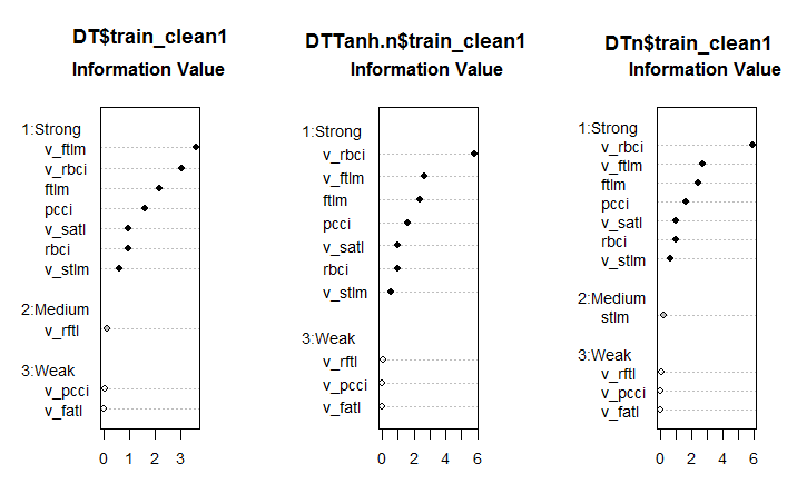
Fig. 6. Importance of predictors in three sets
This is an unexpected result. The v.fatl variable turned out to be the weakest out of the weakest!
The seven strong predictors are the same in all sets. One predictor of a medium power appeared in the first and third sets. This calculation identified the stlm, v.rftl, v.rstl, v.pcci predictors as irrelevant, which is consistent with the earlier calculation. All these computations must be verified by the experiments with an actual model.
The NoiseFilterR package has more than a dozen other filters for identifying noise samples. Happy experimenting!
2. Dimensionality reduction
Dimensionality reduction refers to the transformation of the initial data with a larger dimensionality into a new representation of a smaller dimensionality with keeping main information. Ideally, the dimensionality of the transformed representation is equal to the internal dimensionality of the data. Internal dimensionality of data is the minimal number of variables required for expressing all possible characteristics of data. These are the algorithms traditionally used for reducing dimensionality: Principal Component Analisys (PCA), Independent Component Analisys (ICA) and Singular Value Decomposition (SVD) etc.
Dimensionality reduction allows to soften the so called curse of dimensionality and other undesirable features of high dimensionality spaces. At the stage of describing data, it has the following purposes.
- It reduces computational costs during data processing
- Decreases the need for retraining. The fewer the features, the fewer objects are required for a robust restoration of hidden relationship in the data and the better the quality of restoration of such relationships.
- Compresses data for a more effective storage of information. In such a case, along with the X → T transformation, there must be an opportunity to carry out the inverse transformation T → X
- Data visualization. Projecting a sample onto a two- or three-dimensional space allows to represent this sample graphically
- Extracting new features. New features obtained during the X → T transformation may have a significant impact during the following implementation of solutions for recognition (such as principle component analysis, for instance)
Please note that all methods of dimensionality reductions briefly described below belong to the class of unsupervised training. This means that only the feature description of objects X (predictors) are playing a role of initial information.
2.1. PCA, Principal Component Analysis
Principal component analysis (PCA) is the simplest method of reducing data dimensionality. Main ideas of this method date back to the 19th century. The principle of this method is to find a hyperplane of the set dimension in the initial space and project the data set to this hyperplane. The hyperplane with the smallest error of projecting data (sum of deviations squared) is selected.
The dimensionality of reduced space d can be preset by the user. This value is easy to select if we have a problem of visualizing data (d = 2 or d = 3) or a problem of putting a data set into a set memory. In other cases, the choice of d is not obvious from prior assumptions.
There is a simple heuristic method of selecting the value of d for the method of principal components. One of the peculiarities of the method of principal components is that all reduced spaces for d = 1, 2, . . . are inserted into each other. This way, once all eigenvectors and eigenvalues of the covariance matrix are calculated, we can obtain a reduced space for any value of d. So, to select the d value, the eigenvalues can be shown on the chart in the decreasing order and the cutoff threshold can be set in the way so that the values negligibly different from zero were on the right hand side. Another way to select the d value is to select the threshold so that a certain percent of the total area under the curve stays on the right (for instance, 5% or 1%).
In simple terms, PCA can be treated as a preliminary suppression of noise predictors if their number is significant (>50).
2.2. ICA, Independent Component Analysis
Unlike PCA, independent component analysis is a recent thing, though quickly gaining popularity in various areas of data exploration.
Method of independent components is widely used during signal processing. This technique linearly transforms initial data into new components. The new components will be as statistically independent from each other as possible. Independent components are not necessarily orthogonal but their statistical independence is a more strict condition than the absence of statistical correlation in PCA.
The PCA and ICA methods are implemented in the caret package by the preProcess() function. In this function either the number of principal components or cumulative percent of dispersion covered by PCA can be set. Independent Component Analysis has two stages. At first, required parameters are calculated on the train data set. Then, the data sets and all new data coming in later are transformed using predict().
Table 1. Comparative characteristics of PCA and ICA
| Method | Advantages | Disadvantages | Peculiarities | Result obtained in most cases | Way to calculate new principal components |
|---|---|---|---|---|---|
| PCA | Simplicity of calculations |
| Non-uniqueness of solution (rotational uncertainty). Every new calculation based on one training test will produce different principal components. |
| Tnew = Xnew * P |
| ICA | Simplicity of calculations |
| With a large difference in the dimensionality of the input data set and independent components, used consecutively PCA -> ICA. |
| Snew =scale( Xnew )* W * K |
Let us carry out an experiment. Load the results of script calculations from the first part of the article Part_1.Rda into Rstudio. Below is the content of env:
> ls(env)
 [1] "cap1"         "cap2"         "Close"        "Data"         "dataSet"
 [6] "dataSetCap"   "dataSetClean" "dataSetOut"   "High"         "i"
[11] "k"            "k.cap"        "k.out"        "lof.x"        "lof.x.cap"
[16] "Low"          "lower"        "med"          "Open"         "out.ftlm"
[21] "out.ftlm1"    "pr"           "pre.outl"     "preProClean"  "Rlof.x"
[26] "Rlof.x.cap"   "sk"           "sk.cap"       "sk.out"       "test"
[31] "test.out"     "train"        "train.out"    "upper"        "Volume"
[36] "x"            "x.cap"        "x.out"
Take the x.cap data set with outliers imputed and calculate its principle and independent components using the preProcess::caret function. Specify explicitly the number of components for PCA and ICA. We are not going to specify the way of normalization for ICA.
require(caret)
evalq({
  prePCA <- preProcess(x.cap,
                       pcaComp = 5,
                       method = Hmisc::Cs(center, scale, pca))
  preICA <- preProcess(x.cap,
                       n.comp = 3,
                       method = "ica")
}, env)
Let us look at the parameters of transformation:> str(env$prePCA) List of 20 $ dim : int [1:2] 7906 11 $ bc : NULL $ yj : NULL $ et : NULL $ invHyperbolicSine: NULL $ mean : Named num [1:11] -0.001042 -0.003567 -0.000155 -0.000104 -0.000267 ... ..- attr(*, "names")= chr [1:11] "ftlm" "stlm" "rbci" "pcci" ... $ std : Named num [1:11] 0.091 0.237 0.1023 0.0377 0.0356 ... ..- attr(*, "names")= chr [1:11] "ftlm" "stlm" "rbci" "pcci" ... $ ranges : NULL $ rotation : num [1:11, 1:5] -0.428 -0.091 -0.437 -0.107 -0.32 ... ..- attr(*, "dimnames")=List of 2 .. ..$ : chr [1:11] "ftlm" "stlm" "rbci" "pcci" ... .. ..$ : chr [1:5] "PC1" "PC2" "PC3" "PC4" ... $ method :List of 4 ..$ center: chr [1:11] "ftlm" "stlm" "rbci" "pcci" ... ..$ scale : chr [1:11] "ftlm" "stlm" "rbci" "pcci" ... ..$ pca : chr [1:11] "ftlm" "stlm" "rbci" "pcci" ... ..$ ignore: chr(0) $ thresh : num 0.95 $ pcaComp : num 5 $ numComp : num 5 $ ica : NULL $ wildcards :List of 2 ..$ PCA: chr(0) ..$ ICA: chr(0) $ k : num 5 $ knnSummary :function (x, ...) $ bagImp : NULL $ median : NULL $ data : NULL - attr(*, "class")= chr "preProcess"
We are interested in three slots. They are prePCA$mean, prePCA$std (parameters of normalization) and prePCA$rotation (matrix of rotation and loadings).
> str(env$preICA)
List of 20
 $ dim              : int [1:2] 7906 11
 $ bc               : NULL
 $ yj               : NULL
 $ et               : NULL
 $ invHyperbolicSine: NULL
 $ mean             : Named num [1:11] -0.001042 -0.003567 -0.000155 -0.000104 -0.000267 ...
  ..- attr(*, "names")= chr [1:11] "ftlm" "stlm" "rbci" "pcci" ...
 $ std              : Named num [1:11] 0.091 0.237 0.1023 0.0377 0.0356 ...
  ..- attr(*, "names")= chr [1:11] "ftlm" "stlm" "rbci" "pcci" ...
 $ ranges           : NULL
 $ rotation         : NULL
 $ method           :List of 4
  ..$ ica   : chr [1:11] "ftlm" "stlm" "rbci" "pcci" ...
  ..$ center: chr [1:11] "ftlm" "stlm" "rbci" "pcci" ...
  ..$ scale : chr [1:11] "ftlm" "stlm" "rbci" "pcci" ...
  ..$ ignore: chr(0)
 $ thresh           : num 0.95
 $ pcaComp          : NULL
 $ numComp          : NULL
 $ ica              :List of 3
  ..$ row.norm: logi FALSE
  ..$ K       : num [1:11, 1:3] -0.214 -0.0455 -0.2185 -0.0534 -0.1604 ...
  ..$ W       : num [1:3, 1:3] -0.587 0.77 -0.25 -0.734 -0.636 ...
 $ wildcards        :List of 2
  ..$ PCA: chr(0)
  ..$ ICA: chr(0)
 $ k                : num 5
 $ knnSummary       :function (x, ...)
 $ bagImp           : NULL
 $ median           : NULL
 $ data             : NULL
 - attr(*, "class")= chr "preProcess"
Here we have same $mean and $std and two matrices $K and $W. The caret package for calculating ICA uses the fastICA package with the following algorithm:
- after the initial matrix is centered (normalization of rows is possible), we obtain the Х matrix
- then the Х matrix is projected into the directions of the principle components and we obtain PCA = X * K as a result
- after that, PCA is multiplied by the unmixing matrix and we obtain independent components ICA = X * K * W
Let us calculate PCA and ICA in two ways using the predict::caret function and parameters obtained by the preProcess function.
require(magrittr)
evalq({
  pca <- predict(prePCA, x.cap)
  ica <- predict(preICA, x.cap)
  pca1 <- ((x.cap %>% scale(prePCA$mean, prePCA$std)) %*%
                   prePCA$rotation)
  ica1 <- ((x.cap %>% scale(preICA$mean, preICA$std)) %*%
                   preICA$ica$K) %*% preICA$ica$W
  colnames(ica1) <- colnames(ica1, do.NULL = FALSE, prefix = 'ICA')

},env)
evalq(all_equal(pca, pca1), env)
# [1] TRUE
evalq(all_equal(ica, ica1), env)
# [1] TRUE
The result is identical, which was expected.
Using the pcaPP package is a more reliable way for calculating PCA. This method identifies the principal components more precisely.
The fastICA package contains a lot of additional capabilities and parameters for more a flexible and complete calculation of independent components. I would recommend to use fastICA and not a function in caret.
2.3 Probabilistic principal component analysis (PPCA)
PCA has a probabilistic model - PPCA. Restating this method in probabilistic terms gives a number of advantages.
- An opportunity to use the ЕМ algorithm for searching a solution. The ЕМ algorithm is a more effective calculation procedure in the situation when d ≪ D
- Correct processing of missing values. They are simply added to the list of hidden variables of the probabilistic models. Then the ЕМ algorithm is applied to this model.
- A possibility of transition to the model of mixture distributions which broadens the applicability of the method
- A possibility to use the Bayesian approach to solving problems of selecting a model. In particular, a theoretically justified scheme of selecting the dimensionality of reduced space d can be built (see[24, 25])
- A possibility to generate new objects from the probabilistic model
- For the sake of classification - a possibility to model distributions of separate object classes for further use in the schemes of classification
- The value of likelihood function is a universal criterion which allows to compare different probabilistic models with each other. Specifically, outliers in a data set can be easily identified using the likelihood value.
Similar to the classical model of PCA, the probabilistic model PCA is invariant in relation to the choice of the basis in the hyperplane.
Unlike the classical model of PCA, where only the hyperplane explaining data best of all is restored, the probabilistic model restores the whole model of data variability. Namely, it describes data dispersion in all directions. Therefore, the solution includes not only the direction basis vectors of the hyperplane defined by the eigenvectors of the covariance matrix but also the lengths of these basis vectors.
To use РРСА and other nonlinear methods of obtaining principal compounds, the pcaMethods package can be used.
The pcaMethods package is a set of various realizations of PCA and tools for cross validation and visualization of results. The methods mainly allow to apply PCA to incomplete data sets and therefore they can be used for the evaluation of missing values (NA). The package can be found in the repository Bioconductor and can be installed as described below.
source("https://bioconductor.org/biocLite.R")
biocLite("pcaMethods")
library(pcaMethods)
All methods of the package return the pcaRes general class which contains the result. This gives the user good flexibility. The wrapper function pca() enables access to all required types of РСА through their naming argument. Below is a list of algorithms with a brief description:
- svdPCA is a wrapper function for the standard function prcomp.
- svdImpute is the implementation of the algorithm for imputing NA. This is tolerant to a large number of NA (>10%).
- Probabilistic PCA (ppca). PPCA is tolerant to the number of NA between 10% and 15%.
- Bayesian PCA (bpca). Similar to the probabilistic PCA, this uses the EM approach with the Bayesian model for calculating the probability of restoring the value. This algorithm is tolerant to the relatively large number of missing data (> 10%). Scores and loadings, obtained by this method are different to the ones obtained using an ordinary РСА. This is connected with the fact that BPCA was developed specially for the evaluation of missing values and is based on the variation Bayesian framework (VBF) with automated relevance identification (ARD). This algorithm does not force the orthogonality between loadings. In fact, the authors of BPCA found out that including the orthogonality criterion made predictions worse.
- Inverse nonlinear PCA (NLPCA) is best suited for experiment data where the relationship between predictors and the goal variable is nonlinear. NLPCA is based on training of the decoding part of the associative neural network (autoencoder). Loadings can be seen in the hidden layer of the network. Missing values in the training data are just ignored at the error calculation during back propagation. This way, NLPCA can be used for processing of missing values the same way as for a standard РСА. The only difference is that the loadings P are now represented by a neural network. We will study this way of dimensionality reduction in more detail in the "Autoencoder" section.
- Nipals PCA is a nonlinear evaluation by iterative partial least squares. This is an algorithm in the core of the PLS regression, which can perform PCA with missing values leaving them outside of respective internal products. It is tolerant of a small number (usually, not greater than 5%) of missing data.
- Local least squares (LLS) imputation is the algorithm/function llsImpute() for the evaluation of missing values based on the linear combination of k-nearest neighbors of incomplete variable. Distance between variables is defined as the absolute value of the Pearson, Spearman or Kendall correlation coefficients. The optimal linear combination can be found by solving a local problem of least squares.
In the current implementation, two ways of evaluating missing values are presented. These methods differ slightly. The first way is the limitation of the neighbor search in the subset of full variables. This method is preferable when the number of undefined variables is reasonably low. The second method considers all variables as candidates. Missing values here are at first substituted with the average of the columns. Then this method iterates using current evaluation as the input for the LLS regression till the changes between the new and old evaluation fall below a certain threshold (0,001)
Unfortunately, the topic of this article and its volume do not allow me to write about all suggested algorithms of this brilliant package. We will only look at NLPCA in comparison with the autoencoder later.
2.4. Autoencoder
Autoassociative networks have been widely used since deep neural networks appeared. In one of my previous articles we considered in detail the structure and characteristics of training autoencoders(АЕ), stacked autoencoders, restricted Boltzmann machine (RBM) and others.
Autoencoder is a neural network with one or several hidden layers and the number of neurons in the input layer equal to the number of neurons in the output layer. The main purpose of АЕ is to represent the input data as precisely as possible. Same methods of training, regularization and neuron activation used for standard neural networks are used for AE. A model of AE can be built using any package for constructing neural networks, which allows to extract a matrix of hidden layer weights. We will use the autoencoder package. Example below will help to recall possible AE structures:
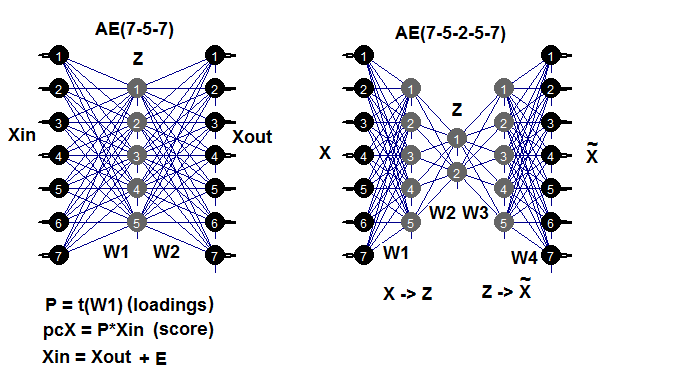
Fig. 7. Structural diagram of autoencoders (three- and five-layer ones)
The weight matrix W1 between the first (input) and the hidden layer is the loading obtained as the result of training. After projecting (multiplication) of the input matrix Xin onto the loading Р, we will obtain a reduced matrix (essentially, principal components). We can get the same result using predict(). This function allows to obtain either the output of the hidden layer (if hidden.output = TRUE) or the output layer of the autoencoder (if hidden.output = FALSE).
After training AE, we can extract the weight matrix W1 and the recovery error from the model. If we input the test data set as well, then we can also obtain the test error from the model. The training error greatly depends on the parameters of AE and even greater from the n.hidden/n.in ratio. The greater this ratio, the greater the recovery error. If we aim to achieve a significant dimensionality reduction, two AE can be connected consequently. For example, if there are 12 inputs we can train a model 12-7-12, perform predict() from the hidden layer and input it to an autoencoder 7-3-7. The reduction will be 12 -> 3. Happy experimenting!
It should be mentioned that although the package claims a capability to create and train a multi-layer AE, I was not able to do it.
Let us conduct an experiment. You already have Part_1.RData with calculation results of the first part of the article. Below is a sequence of calculation:
- create the train/val/test data sets from the dataSet set and obtain the DT list;
- impute outliers and obtain the DTcap list;
- normalize our sets successively using methods with ("center", "scale", "spatialSign"). You can use other methods of transformation and normalization that we considered before;
- train the autoencoder model with three neurons in the hidden layer. You can explore other variants. As the number of hidden neurons increases, the recovery error decreases;
- using the trained model and predict(), obtain the result from the hidden layer. This is essentially a reduced matrix (РСА). Add a goal variable to it;
- plot charts of variation and covariance of the reduced samples train/val/test/.
require(FCNN4R)
require(deepnet)
require(darch)
require(tidyverse)
require(magrittr)
#----Clean---------------------
require(caret)
require(pipeR)
evalq(
  {
    train = 1:2000
    val = 2001:3000
    test = 3001:4000
    DT <- list()
    dataSet %>%
      preProcess(., method = c("zv", "nzv", "conditionalX")) %>%
      predict(., dataSet) %>%
      na.omit -> dataSetClean
    list(train = dataSetClean[train, ],
         val = dataSetClean[val, ],
         test = dataSetClean[test, ]) -> DT
    rm(dataSetClean, train, val, test)
  },
  env)
#------outlier-------------
require(foreach)
evalq({
  DTcap <- list()
  foreach(i = 1:3) %do% {
    DT[[i]] %>%
      select(-c(Data, Class)) %>%
      as.data.frame() -> x
    if (i == 1) {
      foreach(i = 1:ncol(x), .combine = "cbind") %do% {
        prep.outlier(x[ ,i]) %>% unlist()
      } -> pre.outl
      colnames(pre.outl) <- colnames(x)
    }
    foreach(i = 1:ncol(x), .combine = "cbind") %do% {
      stopifnot(exists("pre.outl", envir = env))
      lower = pre.outl['lower.25%', i]
      upper = pre.outl['upper.75%', i]
      med = pre.outl['med', i]
      cap1 = pre.outl['cap1.5%', i]
      cap2 = pre.outl['cap2.95%', i]
      treatOutlier(x = x[ ,i], impute = T, fill = T,
                   lower = lower, upper = upper,
                   med = med, cap1 = cap1, cap2 = cap2)
    } %>% as.data.frame() -> x.cap
    colnames(x.cap) <- colnames(x)
    return(x.cap)
  } -> DTcap
  foreach(i = 1:3) %do% {
    cbind(DTcap[[i]], Class = DT[[i]]$Class)
  } -> DTcap
  DTcap$train <- DTcap[[1]]
  DTcap$val <- DTcap[[2]]
  DTcap$test <- DTcap[[3]]
  rm(lower, upper, med, cap1, cap2, x.cap, x)
}, env)
#------normalize-----------
evalq(
  {
    method <- c("center", "scale", "spatialSign") #, "expoTrans") #"YeoJohnson",
                                                 # "spatialSign"
    preProcess(DTcap$train, method = method) -> preproc
    list(train = predict(preproc, DTcap$train),
         val = predict(preproc, DTcap$val),
         test = predict(preproc, DTcap$test)
    ) -> DTcap.n
    #foreach(i = 1:3) %do% {
    #  cbind(DTcap.n[[i]], Class = DT[[i]]$Class)
    #} -> DTcap.n
  },
  env)
#----train-------
require(autoencoder)
evalq({
  train <-  DTcap.n$train %>% select(-Class) %>% as.matrix()
  val <-  DTcap.n$val %>% select(-Class) %>% as.matrix()
  test <-  DTcap.n$test %>% select(-Class) %>% as.matrix()
  ## Set up the autoencoder architecture:
  nl = 3                    ## number of layers (default is 3: input, hidden, output)
  unit.type = "tanh"        ## specify the network unit type, i.e., the unit's
   ## activation function ("logistic" or "tanh")
  N.input = ncol(train)   ## number of units (neurons) in the input layer (one unit per pixel)
  N.hidden = 3              ## number of units in the hidden layer
  lambda = 0.0002           ## weight decay parameter
  beta = 0                  ## weight of sparsity penalty term
  rho = 0.01                ## desired sparsity parameter
  epsilon <- 0.001          ## a small parameter for initialization of weights
   ## as small gaussian random numbers sampled from N(0,epsilon^2)
  max.iterations = 3000     ## number of iterations in optimizer
   ## Train the autoencoder on training.matrix using BFGS
 ##optimization method
  AE_13 <- autoencode(X.train = train, X.test = val,
                      nl = nl, N.hidden = N.hidden,
                      unit.type = unit.type,
                      lambda = lambda,
                      beta = beta,
                      rho = rho,
                      epsilon = epsilon,
                      optim.method = "BFGS", #"BFGS", "L-BFGS-B", "CG"
                      max.iterations = max.iterations,
                      rescale.flag = FALSE,
                      rescaling.offset = 0.001)}, env)
## Report mean squared error for training and test sets:
#cat("autoencode(): mean squared error for training set: ",
#    round(env$AE_13$mean.error.training.set,3),"\n")
## Extract weights W and biases b from autoencoder.object:
#evalq(P <- AE_13$W, env)
#-----predict-----------
evalq({
  #Train <- predict(AE_13, X.input = train, hidden.output = FALSE)
  pcTrain <- predict(AE_13, X.input = train, hidden.output = TRUE)$X.output %>%
    tbl_df %>% cbind(., Class = DTcap.n$train$Class)
  #Val <- predict(AE_13, X.input = val, hidden.output = FALSE)
  pcVal <- predict(AE_13, X.input = val, hidden.output = TRUE)$X.output %>%
    tbl_df %>% cbind(., Class = DTcap.n$val$Class)
  #Test <- predict(AE_13, X.input = test, hidden.output = FALSE)
  pcTest <- predict(AE_13, X.input = test, hidden.output = TRUE)$X.output %>%
    tbl_df %>% cbind(., Class = DTcap.n$test$Class)
}, env)
#-----graph---------------
require(GGally)
evalq({
  ggpairs(pcTrain,columns = 1:ncol(pcTrain),
          mapping = aes(color = Class),
          title = "pcTrain")},
  env)
evalq({
  ggpairs(pcVal,columns = 1:ncol(pcVal),
          mapping = aes(color = Class),
          title = "pcVal")},
  env)
evalq({
  ggpairs(pcTest,columns = 1:ncol(pcTest),
          mapping = aes(color = Class),
          title = "pcTest")},
  env)
Let us take a look at the charts

Fig. 8. Variation and covariance of the reduced train set
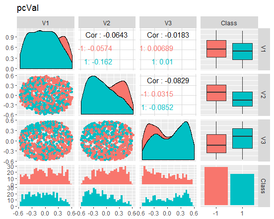
Fig. 9. Variation and covariance of the reduced val set
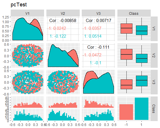
Fig. 10. Variation and covariance of the reduced test set
What do these charts tell us? We can see that the principal components (V1, V2, V3) are divided well by the levels of the goal variable. The distributions in the train/val/test sets are skewed. We should removed noise samples and see if this improves the picture. You can do it on your own.
Small digression: NLPCA
To be able to split data by the principle components, it is important to distinguish applications for pure dimensionality reduction and applications where mainly focusing on the identification and recognition of unique and meaningful components, which is usually called feature extraction.
Applications for pure dimensionality reduction with the accent on suppressing noise and compressing data only require a subspace with high descriptive capacity. The ways separate components make this subspace are not limited and, therefore, do not have to be unique. The only requirement is for the subspace to provide maximum information about mean squared error (MSE). As separate components that cover this subspace are processed by the algorithm without any set order or differentiated weighing, this is called symmetrical training type. This type of training includes a nonlinear PCA, performed by a standard autoassociative neural network (autoencoder), which is therefore called s-NLPCA. In the previous part of the article we considered this variant.
The nonlinear hierarchical PCA (h-NLPCA) provides not only an optimal nonlinear subspace covered by components but also limits nonlinear components by an equal hierarchical order similar to linear components in the standard PCA. The hierarchy in this context is explained by two important properties - scalability and stability. Scalability means that first n components explain maximum dispersion which can be covered by n-dimensional subspace. Stability means that the i-th component of the n-component solution is identical to the i-th component of the m-component solution.
Hierarchical order produces uncorrelated components. The nonlinearity also means that h-NLPCA is capable of removing complex nonlinear correlations between components. This helps to filter useful and meaningful components. Moreover, scaling a nonlinear uncorrelated component to a unit dispersion, we obtain complex nonlinear whitening (spherical transformation). This is a useful preliminary processing for such applications like regression, classification or blind division of sources. Since nonlinear whitening eliminates nonlinear relationships in data, methods used further can be linear. This is especially important for ICA which can be broadened to a nonlinear approach with the use of this nonlinear whitening.
How can we reach a hierarchical order? A simple sorting of symmetrically processed components by dispersion do not produce the required hierarchical order - neither linear, nor nonlinear. A hierarchy can be achieved by two interconnected methods: by either limiting dispersion in the component space or limiting the squared error of reconstruction in the original space. Similar to the linear PCA, i-th component will have to take into consideration the highest i-th dispersion.
In a nonlinear case, this limitation can be ineffective or nonunit without additional limitations. On the contrary, the recovery error can be controlled much better as it is an absolute value invariant to any scaling in a transformation. Therefore, the hierarchical limitation of an error is a more effective method. In a simple linear case, we can achieve the hierarchical arrangement of components by the sequential approach, where components are extracted one by one from the remaining dispersion, defined by the squared error of the previous dispersions. In a nonlinear case, this works neither sequentially nor simultaneously during training several networks in parallel. The remaining dispersion cannot be interpreted by the squared error irrespective of the nonlinear transformation. Solution is in using only one neural network with a hierarchy of sub-networks. This allows us to formulate the hierarchy immediately in the error function.
2.5. Inverse nonlinear PCA
In this part of the article, a nonlinear PCA will be solving a reverse problem. Whereas the original problem is to predict the output from the set input, the reverse problem is the evaluation of the input which best matches a set result. As we know neither the model, nor the process of data generation, we are presented with a so called blind reverse problem.
A simple linear PCA can be considered equally well both in the original and the reverse problems, depending on whether the required components are predicted as outputs or evaluated as input data by a corresponding algorithm. Autoassociative network (АЕ) is modeling the direct and the reverse models simultaneously.
The direct model is defined by the first part of the АЕ by the extracting function Fextr: X → Z. The reverse model is defined by the second part of AE, by the generating function Fgen: Z → X. The first model is better suited for a linear PCA and does not work as well in case of a nonlinear PCA. This happens because this model can be very complex and hard to solve because of the "one-to-many" problem. Two identical sets X can correspond with different values of Z components.
The inverse nonlinear РСА requires only the second part of the autoassociative network (Fig.11), which is illustrated by the network 3-7-12. This part of generation is the reverse reflection of Fgen, which generates or reconstructs big size patterns of Х from their images Z of lower dimensionality. These values of components Z are now unknown inputs which can be evaluated propagating partial errors σ back to the input layer Z.
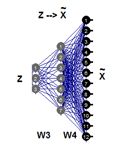
Fig. 11. Inverse nonlinear РСА
Let us compare results obtained with the AE and using the nlpca::pcaMethods function. This function was mentioned earlier in this article. Do the calculation of the same data with the same initial reduction requirement 12->3 and compare results.
For that, take the DTcap.n$train set, remove the goal variable Class and convert it into a matrix. Center the set. Set the structure of the neural network as (3,8,12), the rest of the parameters can be found in the script below. After obtaining the result, single out principal components (scores), add the goal variable to them and plot a chart.
It should be mentioned that this algorithm is very slow and each new launch produces a new result different to the previous one.
require(pcaMethods)
evalq({
  DTcap.n$train %>% tbl_df %>%
    select(-Class) %>% as.matrix() %>%
    prep(scale = "none", center = TRUE) -> train
  resNLPCA <- pca(train,
                  method = "nlpca", weightDecay = 0.01,
                  unitsPerLayer = c(3, 8, 12),
                  center = TRUE, scale = "none",# c("none", "pareto", "vector", "uv")
                  nPcs = 3, completeObs = FALSE,
                  subset = NULL, cv = "none", # "none""q2"), ...)
                  maxSteps = 1100)
  rm(train)},
  env)
#--------
evalq(
   pcTrain <- resNLPCA@scores %>% tbl_df %>%
           cbind(., Class = DTcap.n$train$Class)
, env)
#------graph-------
require(GGally)
evalq({
  ggpairs(pcTrain,columns = 1:ncol(pcTrain),
          mapping = aes(color = Class),
          title = "pcTrain -> NLPCA(3-8-12) wd = 0.01")},
  env)
#----------
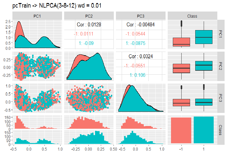
Fig. 12. Variation and covariance of the principle components using NLPCA
What can we see on this chart? Principal components are divided well by the levels of the goal variable and have a very low correlation. The third component looks unnecessary. Let us take a look at the general information on the model.
> print(env$resNLPCA)
nlpca calculated PCA
Importance of component(s):
                 PC1    PC2     PC3
R2            0.3769 0.2718 0.09731
Cumulative R2 0.3769 0.6487 0.74599
12      Variables
2000    Samples
0       NAs ( 0 %)
3       Calculated component(s)
Data was mean centered before running PCA
Data was NOT scaled before running PCA
Scores structure:
[1] 2000    3
Loadings structure:
Inverse hierarchical neural network architecture
3 8 12
Functions in layers
linr tanh linr
hierarchic layer: 1
hierarchic coefficients: 1 1 1 0.01
scaling factor: 0.3260982
There is one problem here. The result does not return weight matrices W3 and W4. In other words, we do not have a loading P and we cannot obtain principal components S (scores) on the test and validation sets. This problem persists in two other decent methods of dimensionality reduction - tSNE, ICS. We could solve these problems reasonably easily but we better not take a route with an unknown outcome.
The package contains two more methods - the probabilistic and Bayesian РСА. They are fast and return loadings, which allows to easily obtain principal components on the validation and test sets. I will bring an example only for PPCA.
#=======PPCA===================
evalq({
  DTcap.n$train %>% tbl_df %>%
    select(-Class) %>% as.matrix() -> train
  DTcap.n$val %>% tbl_df %>%
    select(-Class) %>% as.matrix() -> val
  DTcap.n$test %>% tbl_df %>%
    select(-Class) %>% as.matrix() -> test
  resPPCA <- pca(train, method = "ppca",
                  center = TRUE, scale = "none",# c("none", "pareto", "vector", "uv")
                  nPcs = 3, completeObs = FALSE,
                  subset = NULL, cv = "none", # "none""q2"), ...)
                  maxIterations = 3000)
  },
  env)
#-----------
>print(env$resPPCA)
ppca calculated PCA
Importance of component(s):
 PC1 PC2 PC3
R2 0.2873 0.2499 0.1881
Cumulative R2 0.2873 0.5372 0.7253
12 	Variables
2000 	Samples
0 	NAs ( 0 %)
3 	Calculated component(s)
Data was mean centered before running PCA
Data was NOT scaled before running PCA
Scores structure:
[1] 2000 3
Loadings structure:
[1] 12 3
Plot a chart for loadings and scores for components 1 and 2:
slplot(env$resPPCA, pcs = c(1,2),
       lcex = 0.9, sub = "Probabilistic PCA")
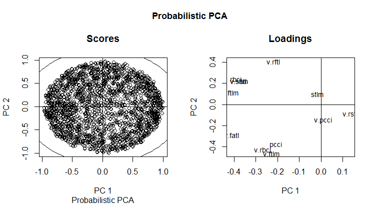
Fig. 13. РС1 and РС2 of the probabilistic РСА (loadings and scores)
Charts of variation and covariance of the principal components of the PPCA train/val/test sets are shown below. You can find the scripts on GitHub.
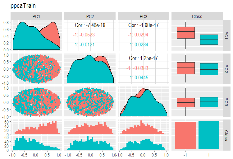
Fig. 14. Variation and covariance of principal components of the train set obtained with PPCA
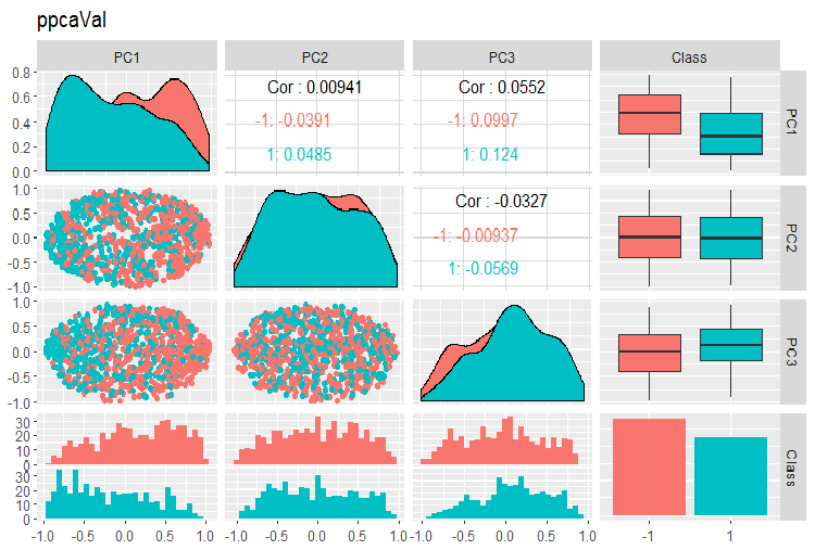
Fig. 15. Variation and covariance of principal components of the val set obtained with PPCA
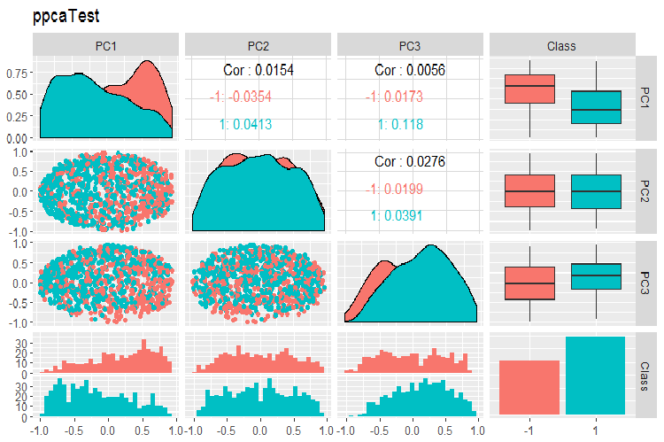
Fig. 16. Variation and covariance of principal components of the test set obtained with PPCA
The division of principal components obtained with PPCA by the levels of the goal variable is not of better quality than same reduction using the autoencoder considered earlier. Advantages of PPCA and BPCA are speed and simplicity. Quality should be evaluated using a certain classification model.
3.Dividing the data set into train/valid/test sets
In this part, everything stays the same as it was described in the previous articles. During training: train/valid/test, sliding window, growing window, sometimes bootstrap. During choosing the model: cross-validation. The matter of identifying a sufficient size of these sets is still an open question.
I would like to mention an interesting statement of Win Wector LLC about using the train sets during preprocessing transformations They say that if principal components have been identified on the training set, the model should be trained on principal components obtained on the validation data set. This means that a used set cannot be used for training a model. This can be tested when the network is trained.
Conclusion
We have considered nearly all stages of data preparation for training deep neural networks. As you can see, this is a complex and time-consuming stage, which requires good theoretical knowledge. Without understanding and skills to prepare data for the following stages, all further actions do not make sense.
It is impossible to reach a good result without a visual control of all calculations at the stage of preparing data. The impatient and lazy will enjoy the "preprocomb" and "metaheur" packages, which will help to find automatically most suitable stages of preliminary preparation.
Application
Scripts used in this article can be found on GitHub/Part_III.
Translated from Russian by MetaQuotes Ltd.
Original article: https://www.mql5.com/ru/articles/3526
 Cross-Platform Expert Advisor: Custom Stops, Breakeven and Trailing
 Using cloud storage services for data exchange between terminals
 Deep Neural Networks (Part IV). Creating, training and testing a model of neural network
- Free trading apps
- Over 8,000 signals for copying
- Economic news for exploring financial markets
You agree to website policy and terms of use