
Deep Neural Networks (Part VII). Ensemble of neural networks: stacking
Contents
- Introduction
- 1. Preparing input data for the trainable combiner
- 2. Base comparison models
- 3. Keras/TensorFlow libraries. General description and installation
- 4. Combiner of bagging ensemble outputs — neural network
- 5. Analysis of experimental results
- Conclusion
- Attachments
Introduction
Models of the base level of the ensemble (individual classifiers) are trained on a full set. Then the metamodel is trained on the ensemble outputs obtained during the prediction based on the testing set. In this case, the outputs of the ensemble's base classifiers become the input data for the new trained classifier, which itself is a combiner. This approach is called "complex combination" or "generalization through learning", more often simply "stacking".
One of the main problems of this combiner is constructing a training set for the metaclassifier.
Let us experiment with the building and testing of stacking ensembles. They will use an ensemble of ELM neural network classifiers with the optimal hyperparameters obtained earlier. Outputs of the pruned ensemble will be used in the first experiment, and all inputs of the ensemble in the second experiment. As combiners, both variants will have fully connected neural networks, but with different structures. In future experiments, we will check how multimodality and multitasking affect the quality of the neural network classification.
Base comparison models will be used to estimate the prediction quality in these variants.
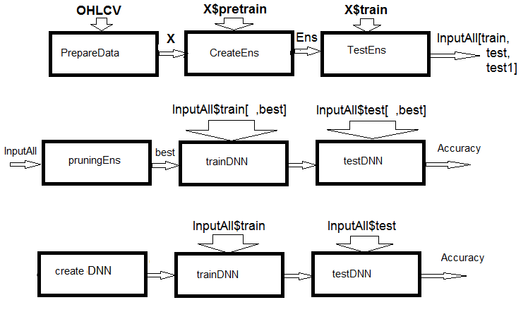
Fig.1. Structural scheme of calculations
As you can see from the figure, the experiment consists of three parts.
- Prepare the input data for the ensemble, train the ELM ensemble and obtain predictions on train/test/test1 sets. These sets will serve as InputAll inputs for the trainable combiners.
- Prune the ensemble: choose the best ELM predictions by information importance. Test the base comparison modules to obtain reference metrics. Train and test the DNN on these data, calculate the metrics of the models and compare them with the metrics of the base model.
- Create a multimodal and multitasking neural networks, train them and test them on the InputAll sets. Calculate the metrics of the obtained models and compare them with the metrics of the base model.
1. Preparing the input data for the trainable combiner
For the experiments, R version 3.4.4 will be used. It contains several new packages which we have not used yet.
Run RStudio. Download the Cotir.RData file containing the terminal quotes from GitHub/Part_I and the Importar.R, Libary.R, FunPrepareData_VII.R, FUN_Stacking.R files with data preparation functions from GitHub/Part_VII. Please note: the sequence of file downloads is important! I have slightly modified the functions to speed up calculations and improve the readability of scripts. Also, added a number of predictors required for the experiments.
We will use the same quotes and split them into the same samples as in the previous articles of this series. Let us write a script for preparing the initial data. The calculation details will not be considered again — they have been described earlier. The changes made are related to using the dplyr package and importing the packages and functions into the working environment. dplyr is a very useful package the facilitates data manipulation. It sometimes presents surprises during debugging, which take many hours of searching for errors.
Let me clarify this. When loading the dplyr library, the following warnings come up in the console:
> library(dplyr)

Attaching package: ‘dplyr’

The following objects are masked from ‘package:stats’:
    filter, lag
The following objects are masked from ‘package:base’:
    intersect, setdiff, setequal, union
A conflict of function names is evident. To solve the problem, it was necessary to explicitly specify the package a specific function is called from. For example, dplyr::filter(), dplyr::lag. The second problem: often, only one or two functions from the package are required, but it is necessary to load the entire library. And certain packages (for example, caret) are massive and are followed by dependent packages that we do not need. In this sense, the style for importing functions and packages in Python is more logical. For example:
from theano import function, config, shared, tensor
import numpy as np
import time
In the first line, a number of functions from the theano package are imported; in the second line, the numpy package is imported and nicknamed np; and in the third — the time package. The same feature in R is implemented in the importar package, which has only two functions — import() and import_fun(). The first one allows you to import packages, and the second one is for importing functions. However, the first one had to be renamed to import_pack(), so that it does not conflict with reticulate::import().
In addition, new variables have been introduced, which will be necessary for the experiments. Generate two data sets — data1 and data2. Arrange their predictors by information importance.
Below is a script for preparing the initial data for the experiments. It is available in the Prepare.R file.
#--0--Library-------------
# source(file = "importar.R")
# source(file = "Library.R")
# source(file = "FunPrepareData_VII.R")
# source(file = "FUN_Stacking.R")
#--1-prepare----
evalq({
  # combine quotes OHLCV, Med, Typ, W into data frame
  # calculate the predictors and the target
  dt <- PrepareData(Data, Open, High, Low, Close, Volume)
  # split the initial data into pretrain/train/val/test
  DT <- SplitData(dt$feature, 4000, 1000, 500, 250, start = 1)
  # define the parameters of outliers
  pre.outl <- PreOutlier(DT$pretrain)
  # impute the outliers in all sets
  DTcap <- CappingData(DT, impute = T, fill = T, dither = F, pre.outl = pre.outl)
  # set the method for normalizing the predictors
  meth <- "spatialSign" #"expoTrans" "range" "spatialSign",
  # define the normalization parameters
  preproc <- PreNorm(DTcap$pretrain, meth = meth, rang = c(-0.95, 0.95))
  # normalize the predictors in all sets
  DTcap.n <- NormData(DTcap, preproc = preproc)
}, env)
In block 0 (Library), load the necessary libraries and functions. Four files with the scripts should be loaded in the specified sequence. In block 1 (prepare), create predictors and normalize them, removing the outliers. The normalization method can be changed.
Now form two data sets — data1 and data2. In the first set, digital filters and their first-order differences will be used as predictors, and the sign of change in the ZigZag's first-order difference serves as the target. In the second set, the predictors will be the first-order differences of the High/Low/Close quotes and the differences of the CO/HO/LO/HL quotes, while the ZigZag's first-order difference will be the target. The script is shown below and is available in the Prepare.R file.
#--2-Data X-------------
evalq({
  foreach(i = 1:length(DTcap)) %do% {
  DTcap.n[[i]] ->.;
  dp$select(., Data, ftlm, stlm, rbci, pcci, fars,
            v.fatl, v.satl, v.rftl, v.rstl,v.ftlm,
            v.stlm, v.rbci, v.pcci, Class)} -> data1
  X1 <- vector(mode = "list", 4)
  foreach(i = 1:length(X1)) %do% {
    data1[[i]] %>% dp$select(-c(Data, Class)) %>% as.data.frame() -> x
    data1[[i]]$Class %>% as.numeric() %>% subtract(1) -> y
    list(x = x, y = y)} -> X1
  list(pretrain = X1[[1]] ,
       train =  X1[[2]] ,
       test =   X1[[3]] ,
       test1 =  X1[[4]] ) -> X1
}, env)
#-----------------
evalq({
  foreach(i = 1:length(DTcap.n)) %do% {
    DTcap.n[[i]] ->.;
    dp$select(., Data, CO, HO, LO, HL, dC, dH, dL)} -> data2
  X2 <- vector(mode = "list", 4)
  foreach(i = 1:length(X2)) %do% {
    data2[[i]] %>% dp$select(-Data) %>% as.data.frame() -> x
    DT[[i]]$dz -> y
    list(x = x, y = y)} -> X2
  list(pretrain = X2[[1]] ,
       train =  X2[[2]] ,
       test =   X2[[3]] ,
       test1 =  X2[[4]] ) -> X2
}, env)
Arrange the predictors in both sets in descending order of their information importance. Let us see how they are ranked. The script is shown below, it is available in the Prepare.R file.
#---3--bestF-----------------------------------
#require(clusterSim)
evalq({
  orderF(x = X1$pretrain$x %>% as.matrix(), type = "metric", s = 1, 4,
         distance =  NULL, # "d1" - Manhattan, "d2" - Euclidean,
         #"d3" - Chebychev (max), "d4" - squared Euclidean,
         #"d5" - GDM1, "d6" - Canberra, "d7" - Bray-Curtis
         method = "kmeans" ,#"kmeans" (default) , "single",
         #"ward.D", "ward.D2", "complete", "average", "mcquitty",
         #"median", "centroid", "pam"
         Index = "cRAND") %$% stopri[ ,1] -> orderX1
}, env)
colnames(env$X1$pretrain$x)[env$orderX1]
[1] "v.fatl" "v.rbci" "v.ftlm" "fars"   "v.satl" "stlm"
[7] "rbci"   "ftlm"   "v.stlm" "v.rftl" "pcci"   "v.rstl"
[13] "v.pcci
evalq({
  orderF(x = X2$pretrain$x %>% as.matrix(), type = "metric", s = 1, 4,
         distance =  NULL, # "d1" - Manhattan, "d2" - Euclidean,
         #"d3" - Chebychev (max), "d4" - squared Euclidean,
         #"d5" - GDM1, "d6" - Canberra, "d7" - Bray-Curtis
         method = "kmeans" ,#"kmeans" (default) , "single",
         #"ward.D", "ward.D2", "complete", "average", "mcquitty",
         #"median", "centroid", "pam"
         Index = "cRAND") %$% stopri[ ,1] -> orderX2
}, env)
colnames(env$X2$pretrain$x)[env$orderX2]
[1] "dC" "CO" "HO" "LO" "dH" "dL" "HL"
The order of the quote predictors is of particular interest.
To prepare the input data for the combiners, it is necessary to:
- create an ELM ensemble and train it on the X1$pretrain training set;
- make a prediction of the X1$train set using the trained ensemble. This will be the InputTrain training set.
- make a prediction of the X1$test set using the trained ensemble. This will be the InputTest testing set;
- make a prediction of the X1$test1 set using the trained ensemble. This will be the InputTest1 testing set.
Define the variables and constants, write the functions createEns() and GetInputData() — it will return the value of all the outputs of the ensemble. Values of the createEns() function parameters have already been obtained after optimization of the ensemble. You may have other values. The script provided below can be found in the FUN_Stacking() file.
#----Library-------------
import_fun(rminer, holdout, holdout)
#source(file = "FunPrepareData_VII.R")
#----Input-------------
evalq({
  #type of activation function.
  Fact <- c("sig", #: sigmoid
            "sin", #: sine
            "radbas", #: radial basis
            "hardlim", #: hard-limit
            "hardlims", #: symmetric hard-limit
            "satlins", #: satlins
            "tansig", #: tan-sigmoid
            "tribas", #: triangular basis
            "poslin", #: positive linear
            "purelin") #: linear
  n <- 500
  #---createENS----------------------
    createEns <- function(numFeature = 8L, r = 7L, nh = 5L, fact = 7L, order, X){
      # determine the indices of the best predictors
      bestF <<- order %>% head(numFeature)
      # choose the best predictors for the training set
      Xtrain <- X$pretrain$x[ , bestF]
      #setMKLthreads(1)
      k <- 1
      rng <- RNGseq(n, 12345)
      #---creste Ensemble---
      Ens <<- foreach(i = 1:n, .packages = "elmNN") %do% {
        rngtools::setRNG(rng[[k]])
        idx <- rminer::holdout(Ytrain, ratio = r/10, mode = "random")$tr
        k <- k + 1
        elmtrain(x = Xtrain[idx, ], y = Ytrain[idx], nhid = nh, actfun = Fact[fact])
      }
      return(Ens)
    }
  #---GetInputData -FUN-----------
  GetInputData <- function(Ens, X){
    #---predict-InputTrain--
    Xtest <- X$train$x[ , bestF]
    foreach(i = 1:n, .packages = "elmNN", .combine = "cbind") %do% {
      predict(Ens[[i]], newdata = Xtest)
    } -> predEns #[ ,n]
    #---predict--InputTest----
    Xtest1 <- X$test$x[ , bestF]
    foreach(i = 1:n, .packages = "elmNN", .combine = "cbind") %do% {
      predict(Ens[[i]], newdata = Xtest1)
    } -> InputTest #[ ,n]
    #---predict--InputTest1----
    Xtest2 <- X$test1$x[ , bestF]
    foreach(i = 1:n, .packages = "elmNN", .combine = "cbind") %do% {
      predict(Ens[[i]], newdata = Xtest2)
    } -> InputTest1 #[ ,n]
    #---res-------------------------
    return(list(InputTrain = predEns,
                InputTest = InputTest,
                InputTest1 = InputTest1))
  }
}, env)
Create an ensemble and calculate the inputs for the trainable combiners:
#---4--createEns----------------
evalq({
  Ytrain <- X1$pretrain$y
  Ytest <- X1$train$y
  Ytest1 <- X1$test$y
  Ytest2 <- X1$test1$y
  Ens <- vector(mode = "list", n)
  createEns(order = orderX1, X = X1) -> Ens
  GetInputData(Ens, X1) -> res
}, env)
Result structure:
> env$res %>% str()
List of 3
 $ InputTrain: num [1:1001, 1:500] 0.811 0.882 0.924 0.817 0.782 ...
 $ InputTest : num [1:501, 1:500] 0.5 0.383 0.366 0.488 0.359 ...
 $ InputTest1: num [1:251, 1:500] 0.32 0.246 0.471 0.563 0.451 ...
2. Base comparison models
Two trainable combiners will be created. One will replace the averaging of outputs of the ensemble's best neural networks, and the second one will replace the pruning and averaging. Therefore, classification quality scores will be required for both options.
Ensemble of neural networks
For the first option, the ELM ensemble with the optimal parameters will be the base comparison model.
Since the second option implies 500 inputs, the varbvs package will be used. It provides fast algorithms to select the Bayesian models for choosing the variables and calculating the Bayesian coefficients, where the result is modeled using linear or logistic regression. These algorithms are based on the variational approximations described in the article "Scalable variational inference for Bayesian variable selection in regression, and its accuracy in genetic association studies". This software was used for work with large data sets containing more than a million variables and thousands of samples.
For the first option, write additional functions getBest(), testAver(), testVot() and calculate the metrics. The functions are available in the FUN_Stacking.R file.
evalq({
  getBest <- function(Ens, x, y, nb){
    n <- length(Ens)
    foreach(i = 1:n, .packages = "elmNN", .combine = "cbind") %do% {
      predict(Ens[[i]], newdata = x)} -> y.pr
    foreach(i = 1:n, .combine = "c") %do% {
      median(y.pr[ ,i])} ->> th
    foreach(i = 1:n, .combine = "c") %do% {
      ifelse(y.pr[ ,i] > th[i], 1, 0) -> Ypred
      Evaluate(actual = y, predicted = Ypred)$Metrics$F1 %>%
        mean()
    } -> Score
    Score %>% order(decreasing = TRUE) %>% head(2*nb + 1) -> best
    y.pr[ ,best] %>%
    apply(1, sum) %>%
    divide_by(length(best)) %>%
    median() -> med
    return(list(Score = Score, bestNN = best, med = med))
  }
  testAver <- function(Ens, x, y, best, med){
    n <- length(Ens)
    foreach(i = 1:n, .packages = "elmNN", .combine = "cbind") %:%
      when(i %in% best) %do% {
        predict(Ens[[i]], newdata = x)} %>%
      apply(1, sum) %>% divide_by(length(best)) -> ensPred
    ifelse(ensPred > med, 1, 0) -> clAver
    Evaluate(actual = y, predicted = clAver)$Metrics[ ,2:5] %>%
      round(3) -> Score
    return(list(Score = Score, Ypred = ensPred, clAver = clAver))
  }
  testVot <- function(Ens, x, y, best){
    n <- length(Ens)
    foreach(i = 1:n, .packages = "elmNN", .combine = "cbind") %:%
      when(i %in% best) %do% {
        predict(Ens[[i]], newdata = x)} %>%
      apply(2, function(x) ifelse(x > th[i], 1, -1)) %>%
      apply(1, function(x) sum(x)) -> vot
    ifelse(vot > 0, 1, 0) -> ClVot
    Evaluate(actual = y, predicted = ClVot)$Metrics[ ,2:5] %>%
      round(3) -> Score
    return(list(Score = Score, Ypred = ClVot))
  }
}, env)
These functions have already been considered. Therefore, we will not dwell on their description. Their outputs, however, are worth noting.
- The function getBest() returns the metrics (Score), the indices of the best individual classifiers of the ensemble (bestNN), the median of the averaged output of the ensemble (med), which will be used when testing the model. The median vector th[500] of all ensemble's outputs is inserted into the environment.
- The function testAver() returns the metrics (Score), the averaged continuous prediction of the ensemble (Ypred) and the nominal prediction of the ensemble (clAver).
- The function testVot() returns the metrics (Score) and the nominal prediction of the ensemble (Ypred).
Test the created ensemble on two testing sets using averaging and majority voting, then see the metrics.
#--2---test----
evalq({
  Ytrain <- X1$pretrain$y
  Ytest <- X1$train$y
  Ytest1 <- X1$test$y
  Ytest2 <- X1$test1$y
  Ens <- vector(mode = "list", n)
  Ens <- createEns(order = orderX1, X = X1)
#---3------
  resBest <- getBest(Ens, x = X1$train$x[ , bestF], y = Ytest, nb = 3)
#---4--averaging---
  ScoreAver <- testAver(Ens, x = X1$test$x[ , bestF], y = Ytest1,
                        best = resBest$bestNN, med = resBest$med)
  ScoreAver1 <- testAver(Ens, x = X1$test1$x[ , bestF], y = Ytest2,
                        best = resBest$bestNN, med = resBest$med)
#---5--voting----
  ScoreVot <- testVot(Ens, x = X1$test$x[ , bestF], y = Ytest1,
                      best = resBest$bestNN)
  ScoreVot1 <- testVot(Ens, x = X1$test1$x[ , bestF], y = Ytest2,
                      best = resBest$bestNN)
}, env)
> env$ScoreAver$Score
  Accuracy Precision Recall    F1
0     0.75     0.708  0.778 0.741
1     0.75     0.794  0.727 0.759
> env$ScoreAver1$Score
  Accuracy Precision Recall    F1
0    0.753     0.750  0.826 0.786
1    0.753     0.758  0.664 0.708
> env$ScoreVot$Score
  Accuracy Precision Recall    F1
0    0.752     0.702  0.800 0.748
1    0.752     0.808  0.712 0.757
> env$ScoreVot1$Score
  Accuracy Precision Recall    F1
0    0.741     0.739  0.819 0.777
1    0.741     0.745  0.646 0.692
Good performance on both testing sets. Below, in analysis of the results, the classification error is decomposed into bias/variance/noise, and the contribution of each component to the total error is estimated.
For the second option (500 inputs), the script for training the model is provided below. It can be found in the varb.R file.
library(varbvs)
evalq({
  vr <- varbvs(X = res$InputTrain, Z = NULL, y = Ytest,
               family = "binomial", optimize.eta = TRUE,
               logodds = seq(-6,-2, 0.25), nr = 250,
               initialize.params = TRUE,
               maxiter = 1e5, verbose = FALSE)
  summary(vr, cred.int = 0.95, nv = 7, nr = 1e5) %>% print()
}, env)
Summary of fitted Bayesian variable selection model:
family:     binomial   num. hyperparameter settings: 17
samples:    1001       iid variable selection prior: yes
variables:  500        fit prior var. of coefs (sa): yes
covariates: 1          fit approx. factors (eta):    yes
maximum log-likelihood lower bound: -579.4602
Hyperparameters:
        estimate Pr>0.95             candidate values
sa          8.09 [7.63,8.54]         NA--NA
logodds    -2.26 [-2.75,-2.00]       (-6.00)--(-2.00)
Selected variables by probability cutoff:
>0.10 >0.25 >0.50 >0.75 >0.90 >0.95
    3     3     3     3     3     3
Top 7 variables by inclusion probability:
     index variable    prob PVE  coef*  Pr(coef.>0.95)
X18     18      X18 1.00000  NA  4.529 [+3.861,+5.195]
X5       5       X5 1.00000  NA  1.955 [+1.543,+2.370]
X255   255     X255 1.00000  NA  2.097 [+1.537,+2.660]
X109   109     X109 0.00948  NA -1.033 [-2.008,-0.057]
X404   404     X404 0.00467  NA -0.665 [-1.350,+0.024]
X275   275     X275 0.00312  NA -0.726 [-1.735,+0.286]
X343   343     X343 0.00299  NA -0.604 [-1.353,+0.149]
*See help(varbvs) about interpreting coefficients in logistic regression.
Using the obtained model, calculate the prediction on two test sets and calculate the metrics.
env$vr$pip %>% order() %>% tail(7) -> bestNN_vr
evalq({
  predict(vr, res$InputTest) -> pr.vr1
  Evaluate(actual = Ytest1, predicted = pr.vr1)$Metrics[ ,2:5] %>%
    round(3) -> metr.test
  confus(table(Ytest1, pr.vr1)) -> cm1
  predict(vr, res$InputTest1) -> pr.vr2
  Evaluate(actual = Ytest2, predicted = pr.vr2)$Metrics[ ,2:5] %>%
    round(3) -> metr.test1
  confus(table(Ytest2, pr.vr2)) -> cm2
}, env)
> env$metr.test
  Accuracy Precision Recall    F1
0     0.78     0.750  0.783 0.766
1     0.78     0.808  0.779 0.793
> env$metr.test1
  Accuracy Precision Recall    F1
0    0.729     0.765  0.732 0.748
1    0.729     0.689  0.726 0.707
The result is excellent, much better than the metrics of the ensemble.
All the data needed to continue the experiments are ready.
Since the keras / tensorflow libraries are to be used in the future, they are briefly considered below.
3. Keras/TensorFlow libraries. General description and installation
The rapidly expanding field of deep neural networks has been supplemented with a number of open source libraries. These include — TensorFlow(Google), CNTK(Microsoft), Apache MXNet and many others. Due to the fact that all these and other major software developers are members of the R Consortium, all these libraries are provided with APIs for R.
All of the above libraries are low-level. They are difficult to learn and use for beginners. With this in mind, the Rstudio team developed the keras package for R.
Keras is a high-level neural network API. The package is designed with an emphasis on the ability to quickly create prototypes and experimentally test a model's performance. Here are the key features of Keras:
- Allows working equally on a CPU or a GPU.
- Friendly API, which allows creating prototypes of deep learning models easily.
- Built-in support for convolutional networks (for computer vision), recurrent networks (for processing sequences) and any combinations thereof.
- Supports arbitrary network architectures: models with multiple inputs or multiple outputs, layer sharing, model sharing, etc. This means that Keras is essentially suitable for constructing any deep learning model, from a memory network to a Neural Turing machine.
- It is able to work on top of several backends, including TensorFlow, CNTK or Theano.
Keras is an API designed for humans, not machines. The package reduces cognitive load: it offers consistent and simple APIs, minimizes the number of user actions and provides effective feedback on user errors. All this makes Keras easy to learn and easy to use. But this is not caused by a decrease in flexibility: since Keras integrates with low-level languages of deep learning (in particular, TensorFlow), it allows you to implement everything that you could create in the base language.
You can develop a Keras model using several deep learning modules. Any Keras model that uses only embedded layers can be transferred among all these backends without changes: you can train a model with one backend and load it in another backend. Available backends include:
- TensorFlow backend (from Google)
- CNTK backend (from Microsoft)
- Theano backend
You can train a Keras model on several different hardware platforms, not just the CPU:
- NVIDIA GPUs
- Google TPUs, via the TensorFlow backend and Google Cloud
- OpenCL-enabled GPUs, such as those from AMD, via the PlaidML Keras backend
Installation of keras and tensorflow backend
Keras and TensorFlow can be configured to work on a CPU or a GPU. The CPU version is much easier to install and set up, therefore, it is the best choice to get started with the package. Here are the manuals for the CPU and GPU versions from the TensorFlow website:
- TensorFlow with CPU support only. If your system does not have a NVIDIA® GPU, you must install this version.
- TensorFlow with GPU support. TensorFlow programs typically run significantly faster on a GPU than on a CPU. Therefore, if your system has a NVIDIA® GPU meeting all prerequisites and you need to run performance-critical applications, you should ultimately install this version.
The only supported installation method on Windows is "conda". This means that you should install Anaconda 3.x (Python 3.5.x/3.6.x) for Windows prior to installing Keras. I installed Anaconda3(Python3.6).
First, install the keras package from CRAN:
install.packages("keras")
The Keras R interface uses TensorFlow by default. To install both the main Keras library and the TensorFlow backend, use the install_keras () function:
# default installation
library(keras)
install_keras()
Thus, CPU versions of Keras and TensorFlow will be installed. If you need a custom setup — for example, with an NVIDIA GPU, see the documentation. To install TensorFlow of a specific version or with GPU support, do the following:
# install with GPU version of TensorFlow
# (NOTE: only do this if you have an NVIDIA GPU + CUDA!)
install_keras(tensorflow = "gpu")

# install a specific version of TensorFlow
install_keras(tensorflow = "1.5")
install_keras(tensorflow = "1.5-gpu")
For more details, see here.
The tfruns supporting package is designed for experiments with TensorFlow. This is a toolkit for managing TensorFlow training and experiments from R.
- Track the hyperparameters, metrics, output data and source code of every training run.
- Compare hyperparameters and metrics across runs to find the best performing model.
- Automatically generate reports to visualize individual training runs or comparisons between runs.
- No changes to source code required (run data is automatically captured for all Keras and tfestimators models).
The best visualization quality of the DNN training process and results are provided by TensorBoard.
Experts in deep learning are given the opportunity to work directly with a low-level TensorFlow library using the tensorflow package.
All these packages are based on the main reticulate package, which is an R interface to Python modules, functions and classes. When called in Python, R data types are automatically converted into their equivalent Python types. The values returned from Python are converted back into R types.
All these packages are well documented, provided with numerous examples, and constantly evolving. This makes it possible to use the most advanced models of deep learning (DNN, RNN, CNN, LSTM, VAE, etc.), reinforcement learning (RL) and many other Python developments in the terminal's experts and indicators. The only limitation is the developer's knowledge and experience.
Here are two more interesting packages worth noting: kerasR and kerasformula. There are tests for the first one, confirming an operation speed higher than that of the original "tensorflow-1.5". The second one offers a simplified version of the model using a formula.
This article only aims to give examples for a simple start in a new field. Its task is not to cover all the diversity of opportunities and get high quality scores of the model.
Before starting the experiments, it is necessary to check if Python is installed and if R interacts with it.
> library(reticulate)
> py_config()
python:         K:\Anaconda3\envs\r-tensorflow\python.exe
libpython:      K:/Anaconda3/envs/r-tensorflow/python36.dll
pythonhome:     K:\ANACON~1\envs\R-TENS~1
version:        3.6.5 | packaged by conda-forge | (default, Apr  6 2018, 16:13:55)
                [MSC v.1900 64 bit (AMD64)]
Architecture:   64bit
numpy:          K:\ANACON~1\envs\R-TENS~1\lib\site-packages\numpy
numpy_version:  1.14.2
tensorflow:     K:\ANACON~1\envs\R-TENS~1\lib\site-packages\tensorflow

python versions found:
 K:\Anaconda3\envs\r-tensorflow\python.exe
 K:\ANACON~1\python.exe
 K:\Anaconda3\python.exe
Let us see the version of tensorflow used:
> library(tensorflow)
> tf_config()
TensorFlow v1.5.1 (K:\ANACON~1\envs\R-TENS~1\lib\site-packages\tensorflow)
Python v3.6 (K:\Anaconda3\envs\r-tensorflow\python.exe)
Everything is ready to continue the experiments.
4. Combiner of bagging ensemble outputs — neural network
Let us perform two experiments. In the first one, apply the softmax function instead of averaging the best outputs of the ensemble. In the second one, replace pruning and averaging by a neural network, feeding all 500 outputs of the ensemble as input. The structure scheme of the experiment is shown in the figure below.
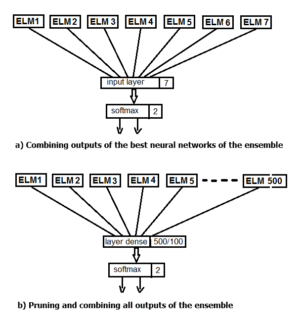
Fig.2. Replacing the averaging of the ensemble outputs with a neural network
The main data structure in Keras is a model, a way of organizing layers. The simplest type is a Sequential model, representing a linear stack of layers.
First, create a simple sequential model, and them start adding layers using the pipe (%>%) operator. For the first experiment, create a neural network, consisting only of the input and output layer. The outputs of the ensemble after pruning, obtained on the testing set, will be fed as input. 20% of the training set will be used for validation. Creation, training and testing of neural networks in this package is extremely easy.
Set the constant parameters of the model, define the training and testing sets for the DNN.
#===========Keras===========================================
library(keras)

num_classes <- 2L
batch_size <- 32L
epochs <- 300L
#---------
bestNN <- env$resBest$bestNN
x_train <- env$res$InputTrain[ ,bestNN]
y_train <- env$Ytest %>% to_categorical()
x_test <- env$res$InputTest[ ,bestNN]
y_test <- env$Ytest1 %>% to_categorical()
x_test1 <- env$res$InputTest1[ ,bestNN]
y_test1 <- env$Ytest2 %>% to_categorical()
Create the model. The script code is provided below. Define and compile a model with structure NN(7, 2) — 7 neurons at input and 2 at output. Optimizer — the "rmsprop" function, loss function — 'binary'_crossentropy', metrics for the test results — "accuracy".
##----model--keras-------------------------
# define model
model <- keras_model_sequential()

# add layers and compile
model %>%
  layer_dense(units = num_classes, input_shape = dim(x_train)[2]) %>%
  layer_activation(activation = 'softmax') %>%
  compile(
    loss = 'binary_crossentropy',
    optimizer =  optimizer_rmsprop(),
    metrics = 'accuracy'
  )
Train and test the model (the script is provided below). Save the history of training. Additionally, specify:
- it is not necessary to output the result of each iteration to the terminal;
- it is not necessary to show real-time charts in Viewer/Rstudio;
- it is necessary to shuffle the input data after each training epoch.
For validation, use 20% of the training set.
## Training & Evaluation ---------------------------
# Fit model to data
model %>% fit(
  x_train, y_train,
  batch_size = batch_size,
  epochs = epochs,
  verbose = 0,
  view_metrics = FALSE,
  shuffle = TRUE,
  validation_split = 0.2) -> history
# Output metrics
score <- model %>% evaluate(x_test, y_test, verbose = 0)
cat('Test loss:', score[[1]] %>% round(3), '\n')
Test loss: 0.518
cat('Test accuracy:', score[[2]] %>% round(3), '\n')
Test accuracy: 0.754
#---------------
score1 <- model %>% evaluate(x_test1, y_test1, verbose = 0)
cat('Test loss:', score1[[1]] %>% round(3), '\n')
Test loss: 0.55
cat('Test accuracy:', score1[[2]] %>% round(3), '\n')
Test accuracy: 0.737
The quantitative results are not bad, they are virtually equal to the ensemble averaging results. Let us see the history of training and testing this model:
#--plot------------------------
plot(history)
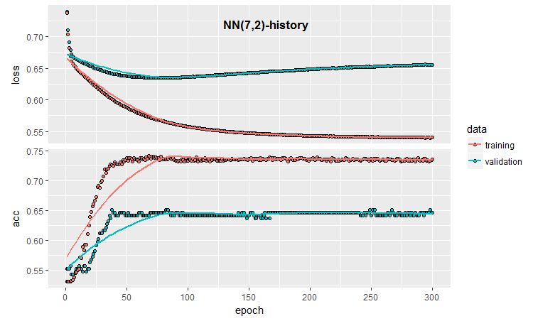
Fig.3. Model training history (7, 2)
The chart shows that the model is clearly overfit after 30 epochs, and after 50 epochs the Accuracy reaches a plateau.
As you remember, the process of neural network initialization is random. That is, each newly created, trained and tested model will produce different results.
Even in this minimal configuration of a neural network, there many opportunities to influence the classification quality and overfitting. Here are some of them: early stopping; neuron initialization method; regularization of the activation function, etc. Of these, we will check only early stopping, adding noise to input data, regularization of the activation function and output a more detailed graphical representation of the training results. To do this, use the ability to apply a callback during the training, provided by keras.
callback_early_stopping(monitor = "val_loss", min_delta = 0, patience = 0,
  verbose = 0, mode = c("auto", "min", "max"))
callback_tensorboard(log_dir = NULL, histogram_freq = 0, batch_size = 32,
  write_graph = TRUE, write_grads = FALSE, write_images = FALSE,
  embeddings_freq = 0, embeddings_layer_names = NULL,
  embeddings_metadata = NULL)
Define the callback functions.
early_stopping <- callback_early_stopping(monitor = "val_acc", min_delta = 1e-5,
                                          patience = 20, verbose = 0,
                                          mode = "auto")
log_dir <- paste0(getwd(),"/run_1")
tensboard <- callback_tensorboard(log_dir = log_dir, histogram_freq = 1,
                                  batch_size = 32, write_graph = TRUE,
                                  write_grads = TRUE, write_images = FALSE)
In the first one, we indicated that it is necessary to track the Accuracy value. If this value becomes less than min_delta in patiente epochs, then the training should be stopped. In the second, we set the path to the directory where the training results should be stored for later playback, and also indicated where to store them exactly. Let us write a complete script using these functions and see the result.
##=====Variant  earlystopping=================================
#--prepare data--------------------------
library(reticulate)
library(keras)
py_set_seed(12345)

num_classes <- 2L
batch_size <- 32L
learning_rate <- 0.005
epochs <- 100L
#---------
bestNN <- env$resBest$bestNN
x_train <- env$res$InputTrain[ ,bestNN]
y_train <- env$Ytest %>% to_categorical()
x_test <- env$res$InputTest[ ,bestNN]
y_test <- env$Ytest1 %>% to_categorical()
x_test1 <- env$res$InputTest1[ ,bestNN]
y_test1 <- env$Ytest2 %>% to_categorical()
##----model--keras-------------------------
# define model
model <- keras_model_sequential()
# add layers and compile
model %>%
  layer_gaussian_noise(stddev = 0.05, input_shape = dim(x_train)[2],
                       name = "GN") %>%
  layer_dense(units = num_classes, name = "dense1") %>%
  layer_activation_softmax(name = "soft") %>%
  layer_activity_regularization(l2 = 1.0, name = "reg") %>%  #l1 = 0.01,
  compile(
    loss = 'binary_crossentropy',
    optimizer =  optimizer_rmsprop(lr = learning_rate, decay = 0.01),
    metrics = 'accuracy'
  )
## Training & Evaluation ---------------------------
# Fit model to data
model %>% fit(
  x_train, y_train,
  batch_size = batch_size,
  epochs = epochs,
  verbose = 0,
  view_metrics = TRUE ,
  shuffle = TRUE,
  validation_split = 0.2,
  callbacks = list(early_stopping, tensboard)) -> history
Metrics on two testing sets and history of training with early stopping.
# Output metrics
> score <- model %>% evaluate(x_test, y_test, verbose = 0)
> cat('Test loss:', score[[1]] %>% round(3), '\n')
Test loss: 0.539
> cat('Test accuracy:', score[[2]] %>% round(3), '\n')
Test accuracy: 0.756
> #---------------
> score1 <- model %>% evaluate(x_test1, y_test1, verbose = 0)
> cat('Test loss:', score1[[1]] %>% round(3), '\n')
Test loss: 0.571
> cat('Test accuracy:', score1[[2]] %>% round(3), '\n')
Test accuracy: 0.713
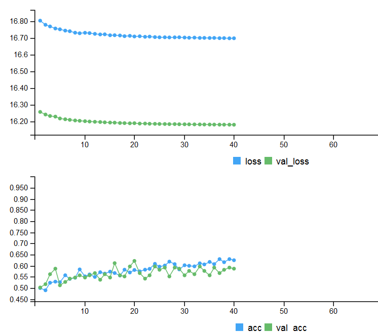
Fig. 4. History of training with early stopping
To display the detailed graphic information about the training process of a neural network, use the tensorboard features:
> tensorboard(log_dir = log_dir)
TensorBoard 1.7.0 at http://127.0.0.1:7451 (Press CTRL+C to quit)
Started TensorBoard at http://127.0.0.1:7451
The browser will open a page where you can view all the internal details of the neural network. Here are sample screenshots:
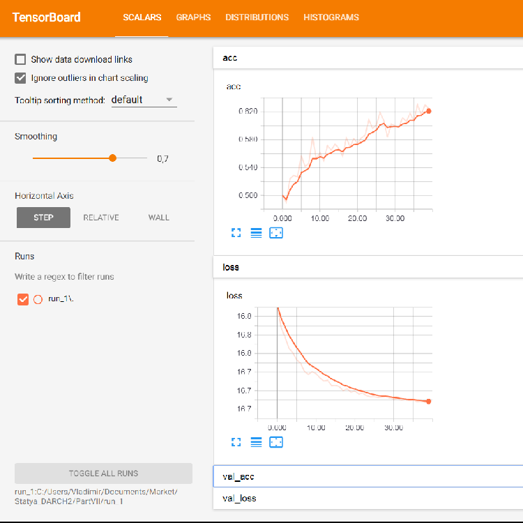
Fig. 5. Loss and accuracy graphs for training on the training set, validation data based on val_acc and val_loss
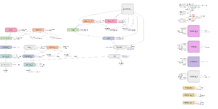
Fig. 6. Computational graph of the neural network
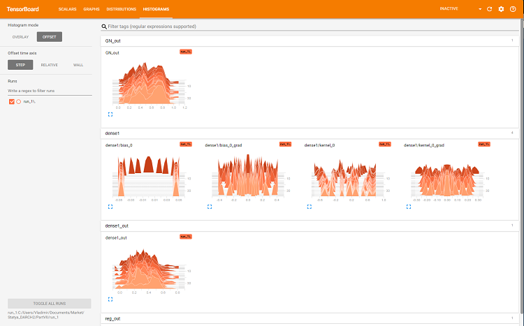
Fig. 7. Histograms of the layer 'dense'
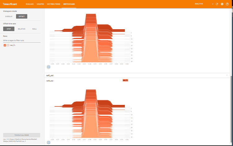
Fig. 8. Histograms of softmax and regularization outputs
These graphs are a powerful tool for adjustment of the neural network's parameters, but their detailed analysis is beyond the scope of this article.
At each new start of tensorboard, it is necessary to change the save path log_dir or to delete the previously used one.
Let us see how the quality of classification with the same parameters would change, but using the testing set for validation. The script is shown below and is available in the file:
library(reticulate)
library(keras)
py_set_seed(12345)

num_classes <- 2L
batch_size <- 32L
learning_rate <- 0.005
epochs <- 100L
#---------
bestNN <- env$resBest$bestNN
x_train <- env$res$InputTrain[ ,bestNN]
y_train <- env$Ytest %>% to_categorical()
x_test <- env$res$InputTest[ ,bestNN]
y_test <- env$Ytest1 %>% to_categorical()
x_test1 <- env$res$InputTest1[ ,bestNN]
y_test1 <- env$Ytest2 %>% to_categorical()
#----------------------------------------
early_stopping <- callback_early_stopping(monitor = "val_acc", min_delta = 1e-5,
                                          patience = 20, verbose = 0,
                                          mode = "auto")
log_dir <- paste0(getwd(),"/run_2")
tensboard <- callback_tensorboard(log_dir = log_dir, histogram_freq = 1,
                                  batch_size = 32, write_graph = TRUE,
                                  write_grads = TRUE, write_images = FALSE)
##----model--keras-------------------------
# define model
model <- keras_model_sequential()
# add layers and compile
model %>%
  layer_gaussian_noise(stddev = 0.05, input_shape = dim(x_train)[2],
                       name = "GN") %>%
  layer_dense(units = num_classes, name = "dense1") %>%
  layer_activation_softmax(name = "soft") %>%
  layer_activity_regularization(l2 = 1.0, name = "reg") %>%  #l1 = 0.01,
  compile(
    loss = 'binary_crossentropy',
    optimizer =  optimizer_rmsprop(lr = learning_rate, decay = 0.01),
    metrics = 'accuracy'
  )
## Training & Evaluation ---------------------------
# Fit model to data
model %>% fit(
  x_train, y_train,
  batch_size = batch_size,
  epochs = epochs,
  verbose = 0,
  view_metrics = TRUE ,
  shuffle = TRUE,
  validation_data = list(x_test, y_test),
  callbacks = list(early_stopping, tensboard)) -> history
Let us see the metrics on the second testing set:
#--model--test1-------------------------------------------------
predict(model, x_test1) -> Ypr.test1
Ypr.test1 %>% max.col()-1 -> y_pr_test1
#Ypr.test1 %>% apply(1, function(x) which.max(x)) %>% subtract(1) -> y_pr_test1
evalq(res_mod_test1 <- Eval(Ytest2, y_pr_test1), env)
> env$res_mod_test1
$metrics
  Accuracy Precision Recall    F1
0    0.713     0.704  0.826 0.760
1    0.713     0.730  0.575 0.644

$confMatr
Confusion Matrix and Statistics

      predicted
actual   0   1
     0 114  24
     1  48  65

               Accuracy : 0.7131
                 95% CI : (0.6529, 0.7683)
    No Information Rate : 0.6454
    P-Value [Acc > NIR] : 0.013728

                  Kappa : 0.4092
 Mcnemar's Test P-Value : 0.006717

            Sensitivity : 0.7037
            Specificity : 0.7303
         Pos Pred Value : 0.8261
         Neg Pred Value : 0.5752
             Prevalence : 0.6454
         Detection Rate : 0.4542
   Detection Prevalence : 0.5498
      Balanced Accuracy : 0.7170

       'Positive' Class : 0
They are virtually identical to those of the first variant. We can visually compare the two variants using tensorboard.
 #-----plot------------------
 tensorboard(log_dir = c(paste0(getwd(),"/run_1"), paste0(getwd(),"/run_2")))
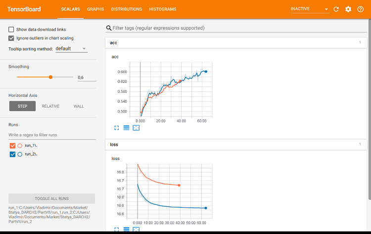
Fig. 9. Metrics on the training set
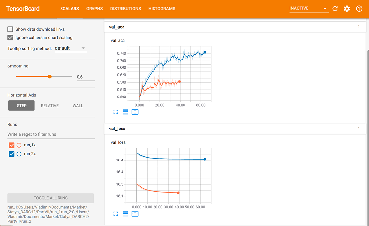
Fig. 10. Metrics on the validation set
This is where differences can be seen.
Let us perform the last experiment. All 500 outputs of the ensemble will be fed as input to the multilayer neural network. Thus, the neural network performs pruning and combination simultaneously. The script is provided below and is also available in the modelDNN_500.R file.
library(reticulate)
library(keras)
py_set_seed(12345)

num_classes <- 2L
batch_size <- 32L
learning_rate <- 0.0001
epochs <- 100L
#---------
x_train <- env$res$InputTrain
y_train <- env$Ytest %>% to_categorical()
x_test <- env$res$InputTest
y_test <- env$Ytest1 %>% to_categorical()
x_test1 <- env$res$InputTest1
y_test1 <- env$Ytest2 %>% to_categorical()
#----------------------------------------
early_stopping <- callback_early_stopping(monitor = "val_acc", min_delta = 1e-5,
                                          patience = 20, verbose = 0,
                                          mode = "auto")
We have loaded the libraries, constants, defined the sets for training and testing, as well as the early stopping function.
##----modelDNN--keras-------------------------
# define model
modDNN <- keras_model_sequential()
# add layers and compile
modDNN %>%
  layer_gaussian_noise(stddev = 0.001, input_shape = dim(x_train)[2], name = "GN") %>%
  layer_batch_normalization() %>%
  layer_dense(units = 100, activation = "elu", name = "dense1") %>%
  layer_dropout(rate = 0.5, name = "dp1") %>%
  layer_batch_normalization() %>%
  layer_dense(units = 50, activation = "elu", name = "dense2") %>%
  layer_batch_normalization() %>%
  layer_dropout(rate = 0.5, name = "dp2") %>%
  layer_dense(units = 10, activation = "elu", name = "dense3") %>%
  layer_batch_normalization() %>%
  layer_dropout(rate = 0.2, name = "dp3") %>%
  layer_dense(units = num_classes, activation = "softmax", name = "soft") %>%
  compile(
    loss = 'binary_crossentropy',
    optimizer =  optimizer_rmsprop(lr = learning_rate, decay = 0.0001),
    metrics = 'accuracy'
  )
So, we have defined the neural network, specifying the sequence and parameters of the layers. We also instructed the compiler on which loss function, optimizer and metric to use when training the model. Now train the model:
## Training & Evaluation ---------------------------
# Fit model to data
modDNN %>% fit(
  x_train, y_train,
  batch_size = batch_size,
  epochs = epochs,
  verbose = 0,
  view_metrics = TRUE ,
  shuffle = TRUE,
  validation_split = 0.2,
  #validation_data = list(x_test, y_test),
  callbacks = list(early_stopping)) -> history
During training, we will output the metrics and shuffle the input data, 20% of the training set will be used for validation, and early stopping will be applied. Test the model on the testing set:
#--model--test-------------------------
predict(modDNN, x_test) -> Ypr.test
Ypr.test %>% apply(1, function(x) which.max(x)) %>% subtract(1) -> y_pr_test
evalq(res_mod_test <- Eval(Ytest1, y_pr_test), env)
It can be seen that the result figures are on par with the ensemble averaging:
> env$res_mod_test
$metrics
  Accuracy Precision Recall    F1
0    0.752     0.702  0.800 0.748
1    0.752     0.808  0.712 0.757

$confMatr
Confusion Matrix and Statistics

      predicted
actual   0   1
     0 184  46
     1  78 193

               Accuracy : 0.7525
                 95% CI : (0.7123, 0.7897)
    No Information Rate : 0.523
    P-Value [Acc > NIR] : < 2.2e-16

                  Kappa : 0.5068
 Mcnemar's Test P-Value : 0.005371

            Sensitivity : 0.7023
            Specificity : 0.8075
         Pos Pred Value : 0.8000
         Neg Pred Value : 0.7122
             Prevalence : 0.5230
         Detection Rate : 0.3673
   Detection Prevalence : 0.4591
      Balanced Accuracy : 0.7549

       'Positive' Class : 0
Let us plot the history of training:
plot(history)
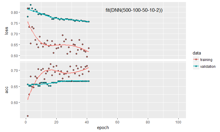
Fig. 11. The history of the DNN500 neural network training
To improve the classification quality, numerous hyperparameters can be modified: neuron initialization method, regularization of activation of the neurons and their weights, etc. The results obtained with almost intuitively selected parameters have a promising quality but also a disappointing cap. Without optimization, it was not possible to raise Accuracy above 0.82. Conclusion: it is necessary to optimize the hyperparameters of the neural network. In the previous articles, we experimented with Bayesian optimization. It can be applied here as well, but it is a separate difficult topic.
Defining a model sequentially allows testing and configuring models of any complexity and depth. But using the functional API of keras, it is possible to create more complex structures of neural networks: for example, with numerous inputs and outputs. This will be discussed in the upcoming article.
5. Analysis of experimental results
So, we have the training and testing results of five models:
- ensemble with averaging (EnsAver);
- ensemble with majority voting (EnsVot);
- logistic regression model varb;
- neural network DNN(7,2);
- neural network DNN500.
Let us gather the quality scores of all these models in one table, decompose the classification error into components and estimate their contribution to the overall error. We use the function randomUniformForest::biasVarCov() (Bias-Variance-Covariance Decomposition). See the package description for more details on this function. The code for decomposition of the classification error of the EnsAver and EnsVot ensembles is shown below. The scripts are similar for other models.
#---bias--test-------------------------------
import_fun(randomUniformForest, biasVarCov, BiasVar)
evalq({
  target = Ytest1
  biasAver <- BiasVar(predictions = ScoreAver$clAver,
                   target = target,
                   regression = FALSE, idx = 1:length(target))
  biasVot <- BiasVar(predictions = ScoreVot$ClVot,
                       target = target,
                       regression = FALSE, idx = 1:length(target))
}, env)
-----------------------------
Noise: 0.2488224
Squared bias: 0.002107561
Variance of estimator: 0.250475
Covariance of estimator and target: 0.1257046

Assuming binary classification with classes {0,1}, where '0' is the majority class.
Misclassification rate = P(Y = 1)P(Y = 0) + {P(Y = 1) - P(Y_hat = 1)}^2 + P(Y_hat = 0)P(Y_hat = 1) - 2*Cov(Y, Y_hat)
Misclassification rate = P(Y = 1) + P(Y_hat = 1) - 2*E(Y*Y_hat) = 0.2499958
---------------------
Noise: 0.2488224
Squared bias: 0.004079665
Variance of estimator: 0.2499721
Covariance of estimator and target: 0.1274411

Assuming binary classification with classes {0,1}, where '0' is the majority class.
Misclassification rate = P(Y = 1)P(Y = 0) + {P(Y = 1) - P(Y_hat = 1)}^2 + P(Y_hat = 0)P(Y_hat = 1) - 2*Cov(Y, Y_hat)
Misclassification rate = P(Y = 1) + P(Y_hat = 1) - 2*E(Y*Y_hat) = 0.2479918
Compact output:
> env$biasAver
$predError
[1] 0.2499958

$squaredBias
[1] 0.002107561

$predictionsVar
[1] 0.250475

$predictionsTargetCov
[1] 0.1257046
| 95%CI Acc | Precision | Recall | F1 | PredErr | sqBias | predVar | predTargCov | |
|---|---|---|---|---|---|---|---|---|
| EnsAver | 0.7102, 0.7880 (0.7500) | 0.708 0.794 |
0.778 0.727 |
0.741 0.759 |
0.2499 | 0.0021 | 0.2505 | 0.1257 |
| EnsVot | 0.7123, 0.7897 (0.7525) | 0.702 0.808 |
0.800 0.712 |
0.748 0.757 |
0.248 | 0.0041 | 0.25 | 0.1274 |
| varb | 0.7416, 0.8159 (0.7804) | 0.790 0.808 |
0.783 0.779 |
0.766 0.793 |
0.2199 | 0.000398 | 0.25 | 0.13964 |
| DNN(7, 2) | 0.7165, 0.7935 (0.7565) | 0.765 0.751 |
0.678 0.823 |
0.719 0.785 |
0.2460 | 0.000195 | 0.2498 | 0.1264 |
| DNN500 | 0.7123, 0.7897 (0.7525) | 0.702 0.808 |
0.800 0.712 |
0.748 0.757 |
0.2779 | 0.01294 | 0.2452 | 0.1145 |
Information in the summary table:
- The best Accuracy score among the base models was obtained by varb, combining 500 outputs of the ensemble. The best model among the trainable combiners according to this score is DNN(7,2), combining 7 best outputs of the ensemble.
- The least test error for the test sample (PredErr) was achieved by varb and DNN(7,2).
- The squared bias (sqBias) of the same two models is an order of magnitude better than the others.
- The error variance (PredVar) of all models is almost the same. This looks strange: the ensemble should have provided a decrease in variance, but we received a low bias.
- The best covariance between the estimate and the response (predictionTargetCov) is shown by varb. It does not mean anything on its own as an individual variable, it is used only for comparing models.
- All scores of the DNN500 model are the lowest. Conclusion: increasing the complexity of models for simple tasks does not lead to better results.
Conclusion
Ensemble of ELM neural network classifiers with averaging or simple majority voting show a good classification quality at very high computational speed. It is possible to improve the quality by optimizing the threshold for converting outputs from continuous to nominal variables and by calibrating the outputs before averaging. No noticeable decrease in variance of the error was detected.
Replacing the averaging of the ensemble outputs with the softmax function of a simple neural network reduces the bias by an order of magnitude without any noticeable decrease in the variance. The use of more complex neural network models for replacing pruning and averaging did not yield good results.
The logistic regression model obtained with the help of Bayesian variable selection (varbvs package) shows very good results. You can use the best outputs determined by this package for the neural network.
24% of noise, which seem to be irremovable since preprocessing, once again prompts that the noise samples should be relabeled to a separate class at some stage.
It is necessary to use the features of keras and to work with sequences (timeseries), which our data are. This can improve the classification quality.
Attachments
GitHub/PartVII contains the following files:
- Importar.R — package import functions.
- Library.R — required libraries.
- FunPrepareData_VII.R — functions for preparing initial data.
- FunStacking.R — functions for creating and testing the ensemble.
- Prepare.R — functions and scripts for preparing the initial data for trainable combiners.
- Varb.R — scripts of the varb base model.
- model_DNN7_2.R — scripts of the DNN(7-2) neural network.
- model_DNN_500.R — scripts of the DNN500 neural network.
- SessionInfo_VII.txt — list of packages used in the article scripts.
Translated from Russian by MetaQuotes Ltd.
Original article: https://www.mql5.com/ru/articles/4228
Warning: All rights to these materials are reserved by MetaQuotes Ltd. Copying or reprinting of these materials in whole or in part is prohibited.
This article was written by a user of the site and reflects their personal views. MetaQuotes Ltd is not responsible for the accuracy of the information presented, nor for any consequences resulting from the use of the solutions, strategies or recommendations described.
 Testing currency pair patterns: Practical application and real trading perspectives. Part IV
 How to create Requirements Specification for ordering a trading robot
 Visualizing optimization results using a selected criterion
 Implementing indicator calculations into an Expert Advisor code
- Free trading apps
- Over 8,000 signals for copying
- Economic news for exploring financial markets
You agree to website policy and terms of use
Vladimir Perervenko
We will build neural networks using the keras/TensorFlow package from Python
What's wrong with R
keras: R Interface to 'Keras'
kerasR: R Interface to the Keras Deep Learning Library.
Greetings CC.
That's the way I use it. keras for R. I tried KerasR, but due to the fact that the tensorflow backend is developing very fast (already version 1.8), it is more reliable to use the package developed and maintained by the Rstudio team.
Good luck
I have plans in the near future to train with reinforcement learning in tandem with neural networks.
Most deliciously, it will be interesting to read your vision of RL application in trading tasks, and realisation of DQN, DDPG, A3C, TRPO
Обсуждение и вопросы по коду можно сделать в ветке
Удачи
Обсуждение и вопросы по коду можно сделать в ветке
Удачи
quick integration with python for deep learning and mt5
https://github.com/TheSnowGuru/PyTrader-python-mt5-trading-api-connector