
Brute force approach to pattern search (Part IV): Minimal functionality
- Changes in the new version
- First demonstration and new concept
- New polynomial based on modified Fourier series
- About software implementation from the inside
- New mechanism for combating spread noise and accounting for spread
- Lot variation on short sections
- Working variants on global history
- Brute force math
- On sticking to history and overfitting
- Recommendations on usage
- Conclusion
- Links to previous articles in the series
Changes in the new version
As in the previous article, the program has been considerably improved in terms of functionality and usability. Previous versions were very inconvenient, had various bugs and errors. This version contains a maximum of changes. A lot has been done to modernize the Expert Advisor templates and the software. List of changes:
- Redesigned interface
- Added another polynomial for brute force (based on the revised Fourier series)
- Enhanced mechanism for generating random numbers
- Extended the method concept towards convenience and ease of use
- Added lot variation mechanisms for ultra-short sections
- Added spread calculation mechanism
- Added a mechanism to reduce spread noise
- Bug fixes
Most of the previously planned modifications have been implemented. Further algorithm amendments will not be so significant.
First demonstration and new concept
While creating EAs, I realized that it might be challenging to always create EA names and deal with numerous settings. Sometimes, names can overlap and settings can be confused. The solution to this problem is an Expert Advisor receiving settings. The program can generate a configuration file in the usual txt format, and the Expert Advisor will read it. This approach speeds up the work with this solution and makes it simpler and more understandable. The solution scheme now looks like this:
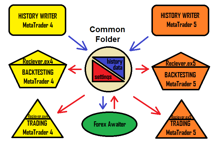
Of course, the version of the program that generates robots is still available. But this article features a new concept invented specifically for the MetaTrader 4 and MetaTrader 5 terminals - it allows ordinary users to start utilizing this solution as simply and quickly as possible. The most convenient part about this solution is that the setting works the same in MetaTrader 4 and in MetaTrader 5.
I will show only part of the new interface, because it is quite large and will take too much space in the article. Here is the first tab.
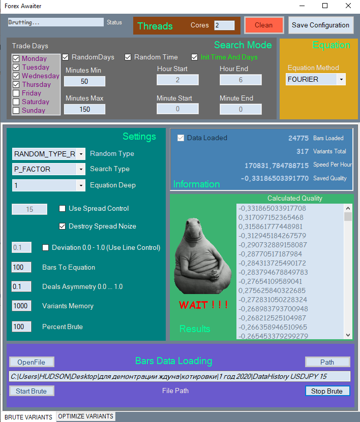
All elements are divided into corresponding sections for easy navigation. Unused elements are blocked if their use is meaningless.
I have created a special video demonstrating the program operation.
Why is it not possible to pass settings via ordinary set files? The reason is that set files cannot contain arrays, while this method uses arrays as inputs which have a floating length. In this case the most convenient solution is to use ordinary text files.
New polynomial based on modified Fourier series
Many people familiar with machine learning actively use the Fourier series for their algorithms for different purposes. The Fourier series was originally created to decompose a function into a series in the range [-π;π]. What we need to know is how to decompose the function into a series and if such decomposition is necessary. In addition, it is important to know the specifics of the variable replacement method, because the decomposition can be performed on a different interval, not in [-π; π]. All this requires good knowledge of mathematics, as the well as understanding of whether there is any purpose of using it for trading. The general view of the Fourier series is as follows:

In this form, this polynomial can only be useful for presenting trading patterns in a more convenient form, as well as for trying to predict price movement, assuming that the price is a wave process. This assumption seems to be valid, but in this form it is inapplicable for brute force, as in this case we would need to radically change the entire concept of the method. Instead, we need to transform the polynomial so that it can be applied for this method. There can be a lot of variations. However, I suggest doing as follows in order to keep the formula close to the Fourier series without using the formula for its intended purpose:

Nothing has changed here, except that the series has more freedom: its period is floating both in plus and minus. Also, there is a finite number of terms now. This is because array C[] contains coefficients which we will combine in an effort to find a suitable formula. The number of such coefficients is limited. This series cannot be infinite, so we have to limit it to "m" bars. Also, I have removed the first term to preserve symmetry - formula values should produce most symmetrical signals in "+" and "-" ranges. But this way can only be used for selecting a function depending on 1 bar! We must ensure that all bar values are available in the formula. Furthermore, a bar has 6 parameters, not 1. These 6 parameters were considered in the second article of this series. Here we have to sacrifice one bar processing accuracy in order to take into account all the rest bars. Ideally, this amount should be wrapped in another one. But I do not want to complicate the polynomial and thus we will use its simplest version for now:

In fact, a one-dimensional function has turned into a multidimensional one. But this does not mean that this polynomial can describe any multidimensional function in the selected multidimensional hypercube. Anyway, this function provides another family of multidimensional functions which can describe other regularities which cannot be properly covered by the Taylor series. This provides more chances of finding a better pattern on the same data sample.
In the code, this function will look like this:
if ( Method == "FOURIER" )
   {
      for ( int i=0; i<CNum; i++ )
         {
         Val+=C1[iterator]*MathSin(C1[iterator+1]*(Close[i+1]-Open[i+1])/_Point)+C1[iterator+2]*MathCos(C1[iterator+3]*(Close[i+1]-Open[i+1])/_Point);
         iterator+=4;
         }

      for ( int i=0; i<CNum; i++ )
         {
         Val+=C1[iterator]*MathSin(C1[iterator+1]*(High[i+1]-Open[i+1])/_Point)+C1[iterator+2]*MathCos(C1[iterator+3]*(High[i+1]-Open[i+1])/_Point);
         iterator+=4;
         }

      for ( int i=0; i<CNum; i++ )
         {
         Val+=C1[iterator]*MathSin(C1[iterator+1]*(Open[i+1]-Low[i+1])/_Point)+C1[iterator+2]*MathCos(C1[iterator+3]*(Open[i+1]-Low[i+1])/_Point);
         iterator+=4;
         }

      for ( int i=0; i<CNum; i++ )
         {
         Val+=C1[iterator]*MathSin(C1[iterator+1]*(High[i+1]-Close[i+1])/_Point)+C1[iterator+2]*MathCos(C1[iterator+3]*(High[i+1]-Close[i+1])/_Point);
         iterator+=4;
         }

      for ( int i=0; i<CNum; i++ )
         {
         Val+=C1[iterator]*MathSin(C1[iterator+1]*(Close[i+1]-Low[i+1])/_Point)+C1[iterator+2]*MathCos(C1[iterator+3]*(Close[i+1]-Low[i+1])/_Point);
         iterator+=4;
         }

   return Val;
   }
It is not the whole function, but only its part which implements the polynomial. Despite the simplicity, even such formulas are adaptable to the market.
I ran a very fast brute force for historical data for the last year using this method to show that this formula can work. However, we will need to find out whether it works good or not. Actually, I haven't managed to find a really efficient solution by using this formula. But I think it is a matter of time and computing capabilities. I spent a lot of time working with the initial version. This is which result I managed to achieve for USDJPY M15 for the last history year:
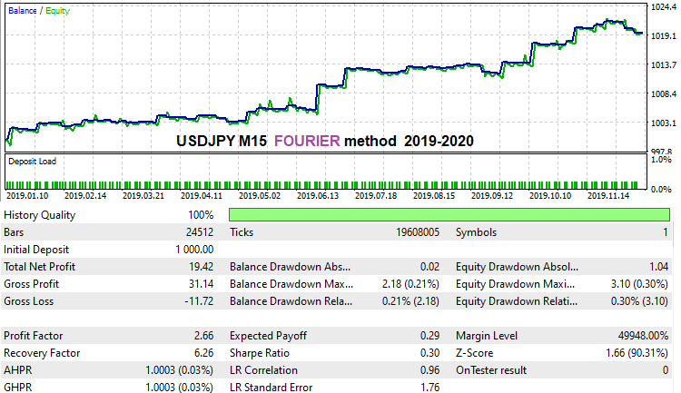
What I didn't like about this formula is that it is very unstable in terms of spread noise suppression. Perhaps this is connected with the specifics of harmonic functions within the framework of this method. Perhaps, I did not quite correctly formulate the formula. Make sure to enable the "Spread Control" option in the second tab. This will disable spread noise suppression mechanism during optimization and produce quite good variants. Probably, the formula is very "gentle". Still, it is able to find pretty good variants.
About software implementation from the inside
These questions had little coverage in my previous articles. I decided to unveil this part to show how it works from the inside. The most interesting and easy part is generating coefficients for the formula. Explanation of this part you can assist you in understanding how the coefficients are generated:
public void GenerateC(Tester CoreWorker)
   {
   double RX;
   TYPE_RANDOM RT;
   RX = RandomX.NextDouble();
   if (RandomType == TYPE_RANDOM.RANDOM_TYPE_R) RT = (TYPE_RANDOM)RandomX.Next(0, Enum.GetValues(typeof(TYPE_RANDOM)).Length-1);
   else RT = RandomType;

   for (int i = 0; i < CoreWorker.Variant.ANum; i++)
      {
      if (RT == TYPE_RANDOM.RANDOM_TYPE_0)
         {
         if (i > 0) CoreWorker.Variant.Ci[i] = CoreWorker.Variant.Ci[i-1]*RandomX.NextDouble();
         else CoreWorker.Variant.Ci[0]=1.0;
         }
      if (RT == TYPE_RANDOM.RANDOM_TYPE_5)
         {
         if (RandomX.NextDouble() >= 0.5)
            {
            if (i > 0) CoreWorker.Variant.Ci[i] = CoreWorker.Variant.Ci[i - 1] * RandomX.NextDouble();
            else CoreWorker.Variant.Ci[0] = 1.0;
            }
         else
            {
            if (i > 0) CoreWorker.Variant.Ci[i] = CoreWorker.Variant.Ci[i - 1] * (-RandomX.NextDouble());
            else CoreWorker.Variant.Ci[0] = -1.0;
            }
         }
      if (RT == TYPE_RANDOM.RANDOM_TYPE_1) CoreWorker.Variant.Ci[i] = RandomX.NextDouble();
      if (RT == TYPE_RANDOM.RANDOM_TYPE_2)
         {
         if (RandomX.NextDouble() >= 0.5) CoreWorker.Variant.Ci[i] = RandomX.NextDouble();
         else CoreWorker.Variant.Ci[i] = -RandomX.NextDouble();
         }
      if (RT == TYPE_RANDOM.RANDOM_TYPE_3)
         {
         if (RandomX.NextDouble() >= RX)
            {
            if (RandomX.NextDouble() >= RX + (1.0 - RX) / 2.0) CoreWorker.Variant.Ci[i] = RandomX.NextDouble();
            else CoreWorker.Variant.Ci[i] = -RandomX.NextDouble();
            }
         else CoreWorker.Variant.Ci[i] = 0.0;
         }
      if (RT == TYPE_RANDOM.RANDOM_TYPE_4)
         {
         if (RandomX.NextDouble() >= RX) CoreWorker.Variant.Ci[i] = RandomX.NextDouble();
         else CoreWorker.Variant.Ci[i] = 0.0;
         }
      }
   }
It is pretty simple: there are several fixed types of random number generation and there is a general type that implements everything at once. Each of the generation types has been tested in practice. It turned out that the general generation type "RANDOM_TYPE_R" shows the maximum efficiency. Fixed types do not always give a result due to the different nature of quotes on different instruments and timeframes. Visually, in most cases, these differences cannot be seen, but the machine sees everything. Although some fixed types on some timeframes can provide more signals with maximum quality. I noticed that, for example, on NZDUSD H1, there is a sharp surge in the quality of results when using RANDOM_TYPE_4, which means "only zeros and positive numbers". This may be a clear hint of hidden wave processes inaccessible to the eye. I would like to explore different instruments in more detail, but it is hard to do alone.
New mechanism for combating spread noise and accounting for spread
As noted in the previous article, spread distorts the price data so that most of the found patterns mostly lie within the spread. The spread is the worst enemy of any strategy, because most strategies fail to provide sufficient mathematical expectation in order to cover the spread. You should not be fooled by a backtest or positive trade statistics on a real account a month or even a year long, because this data sample is too small to assess future performance. There is a separate class of trading strategies and automated trading systems called "Night Scalpers". These robots catch small profit in a limited period of time. Brokers are actively combating such systems by widening spreads after midnight. The spread is set at such a level that most strategies become unprofitable.
There is one value that is almost the same for most brokers:
- Spread = (Ask - Bid) / _Point
- MidPrice = ( Ask + Bid ) / 2
This price is highlighted in green. This is the middle of the order book. The order book is usually lined up relative to this price, and both prices are at an equal distance from this price. In fact, if we look at the classical definition of the order book, this price does not make any sense, since there are no trading orders. Even if we assume that all brokers have their own spreads, this price can be almost the same for all brokers. Here is a diagram:
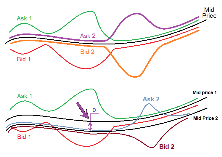
The upper figure shows the price series of two randomly chosen brokers. There is always an "Ask" price and a "Bid" price, which symbolize buying and selling prices. The black line is the same for both price ranges. This price can be calculated easily, as I have shown above. The most important thing is that this value practically does not depend on widened or tightened spreads of a particular broker, since all changes are almost even, relative to a given price.
The lower figure shows a real situation which actually happens with quotes from different brokers. The thing is that even this average price is different in different streams. I do not know the reasons. Even if I knew, this would hardly be useful for trading. I discovered this fact when I was practicing arbitrage trading, where all these nuances are extremely important. In relation to our method, it is only important:
- MidPrice1=f(t)
- MidPrice2=MidPrice1-D
- MidPrice1 '(t) = MidPrice2 '(t)
In other words, the average price of both price series (if represented as time functions) has the same derivative, since these functions differ only in the constant "D". Since our polynomial uses not the prices but their difference, all values will be functionals of the derivative of these average price functions. Since these derivatives are the same for all brokers, we can expect that the settings can be efficient with different brokers. For an alternative case, the found settings will have an extremely low chance of successful backtest on real ticks or of applicability for other brokers. The above concept avoids such problems.
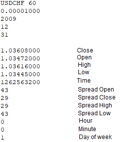
To implement this mechanism, I had to make appropriate modifications of all elements. First, it is necessary to record spreads at all important bar points when writing the quote file. These are the points of Open[], Close[], High[], Low[]. The spread will be used to adjust the values and thus to obtain the Ask price, as bars are based on Bid prices. The EAs which write quotes are based on ticks not bars now. The function for recording these bars looks as follows now:
void WriteBar()
   {
   FileWriteString(Handle0x,"\r\n");
   FileWriteString(Handle0x,DoubleToString(Close[1],8)+"\r\n");
   FileWriteString(Handle0x,DoubleToString(Open[1],8)+"\r\n");
   FileWriteString(Handle0x,DoubleToString(High[1],8)+"\r\n");
   FileWriteString(Handle0x,DoubleToString(Low[1],8)+"\r\n");
   FileWriteString(Handle0x,IntegerToString(int(Time[1]))+"\r\n");
   FileWriteString(Handle0x,IntegerToString(PrevSpread)+"\r\n");
   FileWriteString(Handle0x,IntegerToString(CurrentSpread)+"\r\n");
   FileWriteString(Handle0x,IntegerToString(PrevHighSpread)+"\r\n");
   FileWriteString(Handle0x,IntegerToString(PrevLowSpread)+"\r\n");
   MqlDateTime T;
   TimeToStruct(Time[1],T);
   FileWriteString(Handle0x,IntegerToString(int(T.hour))+"\r\n");
   FileWriteString(Handle0x,IntegerToString(int(T.min))+"\r\n");
   FileWriteString(Handle0x,IntegerToString(int(T.day_of_week))+"\r\n");
   }
Four lines are highlighted in green - these lines record the spread at all four points of the bar. In the previous version, these values were not recorded and were not taken into account in the calculations. These data can be easily obtained and recorded. The following simple tick-based function is used for obtaining the spread at High and Low:
void RecalcHighLowSpreads()
   {
   if ( Close[0] > LastHigh )
      {
      LastHigh=Close[0];
      HighSpread=int(SymbolInfoInteger(_Symbol,SYMBOL_SPREAD));
      }
   if ( Close[0] < LastLow )
      {
      LastLow=Close[0];
      LowSpread=int(SymbolInfoInteger(_Symbol,SYMBOL_SPREAD));
      }
   }
This function only determines the spread at the highest and lowest point of the bar while the current bar is being formed. When a new bar appears, the current bar is considered fully formed and its data is written to the file. This function works in tandem with another bar-based function:
bool bNewBar()
   {
   ArraySetAsSeries(Close,false);
   ArraySetAsSeries(Open,false);
   ArraySetAsSeries(High,false);
   ArraySetAsSeries(Low,false);
   CopyOpen(_Symbol,_Period,0,2,Open);
   CopyClose(_Symbol,_Period,0,2,Close);
   CopyHigh(_Symbol,_Period,0,2,High);
   CopyLow(_Symbol,_Period,0,2,Low);
   ArraySetAsSeries(Close,true);
   ArraySetAsSeries(Open,true);
   ArraySetAsSeries(High,true);
   ArraySetAsSeries(Low,true);
   if ( Time0 < Time[1] )
      {
      if (Time0 != 0)
         {
         Time0=Time[1];
         PrevHighSpread=HighSpread;
         PrevLowSpread=LowSpread;
         PrevSpread=CurrentSpread;
         CurrentSpread=int(SymbolInfoInteger(_Symbol,SYMBOL_SPREAD));
         HighSpread=CurrentSpread;
         LowSpread=CurrentSpread;
         return true;
         }
      else
         {
         Time0=Time[1];
         return false;
         }
      }
   else return false;
   }
The function is both a predicate and an important element of logic, in which all four spreads are finally determined. It is similarly implemented inside the program. It works very simply in the OnTick handler:
RecalcHighLowSpreads();
if ( bNewBar()) WriteBar();
The quote file will contain the following data:
An array with average prices is implemented identically inside the program:
OpenX[1]=Open[1]+(double(PrevSpread)/2.0)*_Point;
CloseX[1]=Close[1]+(double(Spread)/2.0)*_Point;
HighX[1]=High[1]+(double(PrevHighSpread)/2.0)*_Point;
LowX[1]=Low[1]+(double(PrevLowSpread)/2.0)*_Point;
It may seem that this approach can be used to implement suppression of spread noise. However, the problem is that it requires a certain number of collected ticks (the higher the timeframe, the more ticks are needed per bar). Collection of a large number of ticks requires much time. Furthermore, bars do not store Ask prices or spread values, that is why we used Bid for calculations.
As an additional option, I have added a mechanism to take into account the spread when optimizing results. Tests have shown that this mechanism is optional, but with sufficient computing power, it can give quite good results. The point is to require the algorithm to open and close orders only if the spread does not exceed the required value. The current version records spreads into bar data, so the value can be controlled, allowing us to calculate the true test values excluding the spread.
Lot variation on short sections
Lot variation (one of the varieties) can be used not only on very short sections, but also on long ones. There are two risk/lot management mechanisms.
- Lot increase
- Lot decrease
The first mechanism should be used in inverted trading, when we expect the signal to be inverted soon. The second option only works if it is known that the signal is stable and will last for a long time. You can use any control functions. I used the simplest ones — linear functions. In other words, lots change over time. Let us view the mechanism operation in practice.
This will be done using the USDJPY M15 quote. In this case, I use the MQL4 version of the robot for demonstration, since the robot fails backtests on real ticks as it trades at increased-spread points. I wanted to prove that a good brute force approach on low timeframes can provide good forward results in an interval equal to the brute force period and more. The work was not very broad since my computing capacities are limited. But this result is quite enough to demonstrate a fairly long working forward period, with two lot management mechanisms in these forward sections. Let us start with a demonstration of the found variant in the search interval. The interval is equal to one year:
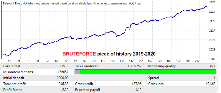
The mathematical expectation here is a little more than 12 points (without spread this time, which is not important to us as we ignore spread this time). We will look at the profit factor. A one-year forward test looks as follows:
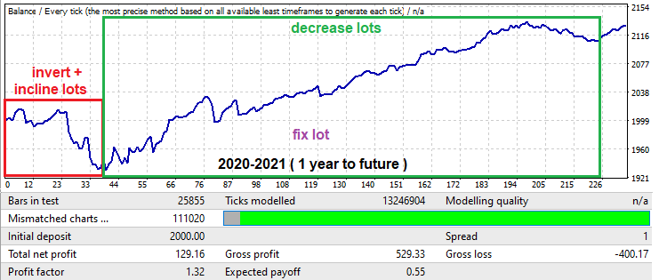
Despite the fact that the search took only one year, it continued to work for no less than one year. In practice, this means that if you have a good computer, you can analyze all major currency pairs with low spreads in a week or two, then choose the best of them and exploit the pattern for at least another year. Do not forget to make sure that the system passes a real-tick backtest in MetaTrader 5. To collect even more evidence, it is a good idea to join into a small team to analyze data on several computers in order to collect results and compile statistics.
Now let us look at the forward test - at the beginning there is a very large drawdown, which is usually very common when we are looking for patterns in small time periods such as one year. Nevertheless, even this drawdown can be used for your own purposes. This interval is shown in a red frame in the above graph. The EA working time here is limited in the settings to 50 trading days (Saturday and Sunday are not counted). Also, the signal was inverted to turn the drawdown into a profit. This is done to cut off the graph part after the drawdown since it would turn into a negative one after inversion. The resulting backtest is as follows:
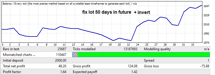
Pay attention to the profit factor. We are going to increase it. You never really know if there will be a reversal and how far that reversal will go, but it usually rolls back by a fairly large portion of the movement that occurred in the brute force segment. By applying a linear gain of the lot from the minimum to the maximum, we will get such a backtest and an increase in the profit factor:
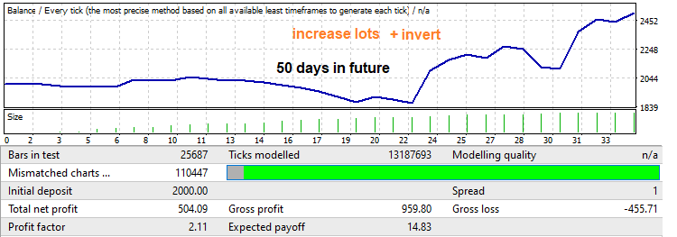
Now let us see the reverse mechanism, which is shown in a green frame in the one-year forward test. This part shows a large growing part followed by a pattern reversal. In this situation we will use lot decrease. The robot is set to trade up to the end of this segment. First, let us test it with a fixed lot to be able to compare the results later:
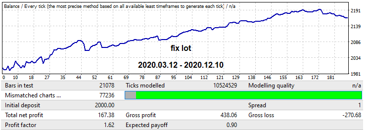
Now let us enable the mechanism that implements lot decrease over time. This also produces an increase in the profit factor, while the graph becomes smoother and there is no drawdown at the end:
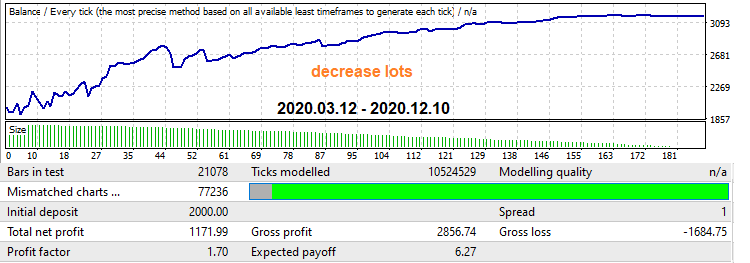
Many Market sellers use these techniques. When applied at the right time and in the right place, they can both increase profitability and reduce losses. In practice it is more complicated though. Anyway, these mechanisms are provided in the Expert Advisors generated by my program, so you can enable and disable them whenever needed.
Working variants on global history
I think many readers would be interested to see and check at least some working settings variants which are able to pass global backtests on real tick history. I have found such settings. Due to the limited computing capabilities and because I perform brute force alone, search took quite a long time. Nevertheless, I have found some variants. Here they are:
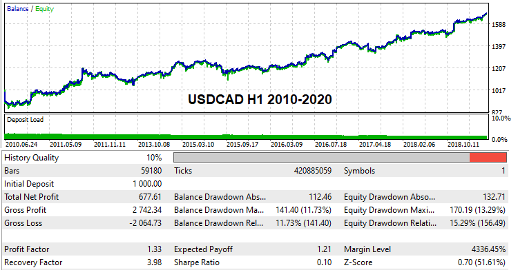
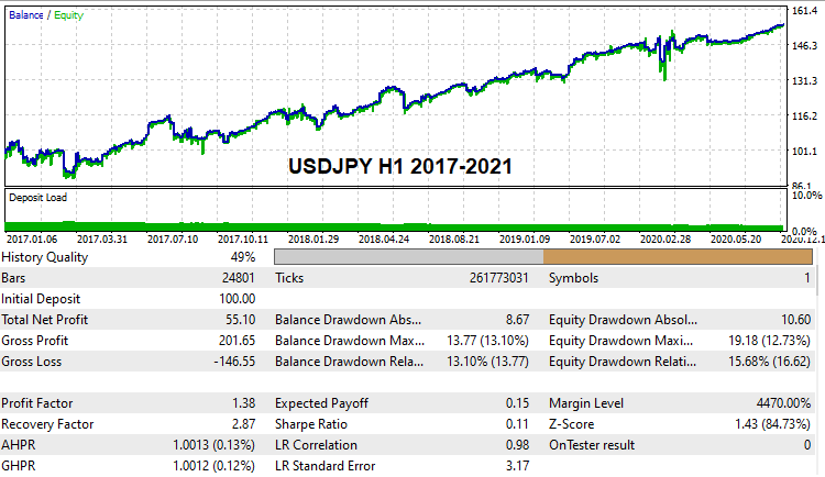
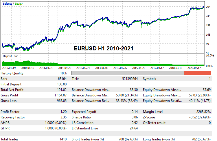
These settings are attached below, so you can test them if you wish. You can also try to find your own settings and backtest them on demo accounts. Starting with this version of the program, anyone can try this method.
Brute force math
This section needs thorough explanation to help users understand the underlying calculation principles. Let us begin with how the first tab of the program works and how to interpret its results.
Brute force in the first tab
In fact, everything that happens in any brute force algorithm is always connected with the theory of probability, because we always have some kind of model and an iteration. An iteration here is a full cycle of the analysis of the current strategy variant. A full cycle can consist of one test or multiple ones, depending on the specific approach. The number of tests and other manipulations is not so important as everything can be classified as one iteration. An iteration can be considered successful or unsuccessful, depending on the requirements for the result. A wide variety of quantitative values can serve as criteria for a good result, which depends on the analysis method.
The algorithm always outputs one or more variants that fit our requirements. We can instruct the algorithm on how much results should be stored in memory. All other results which meet the requirement but do not fit into the storage will be discarded. No matter how many steps there are in our brute force algorithm, this process will always take place. Otherwise, we would waste too much time processing deliberately low-quality data. This way, not a single variant will be lost, but this can reduce the search speed. Which approach to use is ultimately up to you.
Now let us get straight to the point. Any result searching process ultimately comes down to a process of independent tests according to the Bernoulli scheme (provided that the algorithm is fixed). It all depends on the likelihood of getting a good variant. This probability is always fixed for a fixed algorithm. In our case, this probability depends on the following values:
- Sample size
- Algorithm variability
- Proximity to the base
- Strictness of requirements for the final result
In this regard, the quantity and quality of the results obtained grow with the number of iterations, according to the Bernoulli formula. However, do not forget that this is a purely probabilistic process! That is, it is impossible to predict for sure which set of results you will obtain. It is only possible to calculate the probability of finding the desired result
- Pk - the probability that the iteration will produce a working variant with the specified requirements (this probability can vary greatly depending on the requirements)
- C(n,m) - the number of "n" to "m" combinations
- Pa=Sum(m0...m...n)[C(n,m)*Pow(Pk ,m)*Pow(1-Pk ,n-m)] - the probability that after n iterations we will have at least m0 primary variants meeting our requirements
- m0 - minimum number of satisfactory prototypes
- Pa — probability of obtaining at least "m0" or more from "n" iterations
- n — maximum available number of cycles of searching for working prototypes (how long we are ready to wait for the results)
The number of cycles can also be expressed in terms of time: take the speed of brute force from the counter in the first tab and the time that you are ready to spend on processing the current data:
- Sh - speed as the number of iterations per hour
- T - time in hours which we are ready to wait
- n = Sh*T
In a similar it is possible to calculate the probability of finding variants in accordance with certain quality requirements. The above formulas allowed finding variants that fall under the "Deviation" filter, which is a requirement for the linearity of the result. If this filter is not enabled, each iteration will be considered successful and there will always be variants. Found variants will be sorted by quality score. Depending on the needed quality, the "Ps" value will be a function of the quality value taken modulo. The higher the quality we need, the lower the value of this function:
- Ps - the probability of finding a result with certain additional quality requirements
- q - the required quality
- qMax - the highest available quality
- Ps = Ps(|q|) = K * Px(|q|) , q <= qMax
- K = Pk - this coefficient takes into account the probability of obtaining some random variant (quality-based variants are selected from such variants)
- Ps ' (|q|) < 0
- Lim (q-->qMax) [ Ps(|q|) ] = 0
The first derivative of this function is negative, symbolizing that as the requirements increase, the probability of meeting them tends to zero. When "q" tends to the maximum available value, the value of this function tends to "0", since this is a probability. If "q" is greater than the maximum value, this function is meaningless, since the selected algorithm cannot each a higher quality. This function follows from the probability density function of a random variable "q". The below figure shows Ps(q) and the probability density of the random variable P(q), as well as additional important quantities:
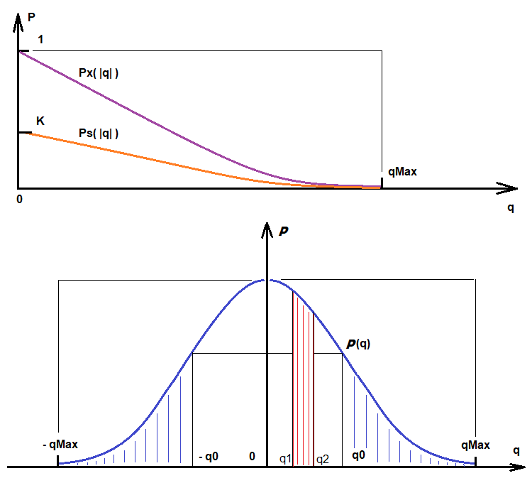
Based on these illustrations:
- Integral(q0,qMax) [P(q)] = Integral(-qMax,-q0) [P(q)] = K*Px(|q|) = Ps(|q|) - this is the probability that a variant with |q| between q0 and qMax will be found during the current iteration.
- Integral(q1,q2) [P(q)] - the probability that a quality value between q1 and q2 will be obtained as a result of the iteration (this is an example of how to interpret the random variable distribution function)
So, the more quality we want, the more time we have to spend and the fewer variants will be found. In addition, any method has an upper limit on the quality value, which depends both on the data that we analyze and on the perfection of our method.
Optimization in the second tab
The optimization process in the second tab is slightly different from the primary search process. Anyway, it still uses an iteration and the probability of obtaining a variant that meets our requirements. This tab has much more filters, accordingly, the probability of obtaining good results is lower. However, since the second tab improves already processed variants, the better the options found in the first tab, the better results will be obtained on the second one. The final formula according to which a certain variant is improved is somewhat similar to the Bernoulli equation. What we are interested in is the probability of obtaining at least one variant that falls under our filters. An explanation follows:
- Py = Sum(1...m...n)[ Sum(0... i ... C(n,m)-1) { Product(0 .. j .. i-1 )[Pk[j]) * Product(i .. j .. m) [1 - Pk[j]] } ] - the probability of obtaining at least one variant that meets filter requirements
- Pk [i] - probability of obtaining a variant that meets the requirements of filters in the second tab
- n - splitting the optimization interval (Interval Points value in the 2nd tab)
Optimization is performed in exactly the same way as in the MetaTrader 4 and MetaTrader 5 optimizers, however we only optimize one parameter which is a buy or sell signal. The optimization step is calculated automatically, based on how many parts we divide the optimization interval (Interval Points). The highest value of the number being optimized is calculated during the search process in the first tab. After the process in the first tab has completed, we know the range of fluctuations in the values of the optimized number. So, in the second tab, we only need to set the grid accuracy to split this interval. The variant takes one slot in the second tab, which will be updated whenever a better quality is achieved.
Again, the probability of obtaining some variant with quality requirements will have some distribution function similar to the one above. it means that we can use the same formulas with a slight adjustment:
- Integral(q0,qMax) [P(q)] = Integral(-qMax,-q0) [P(q)] = K*Px(|q|) = Pz(|q|) - this is the probability that a variant with |q| between q0 and qMax will be found during the current iteration.
- K = Py
The only difference here is the coefficient "K", which is equal to the new probability obtained earlier. The probability of obtaining a variant of the required quality is very low, but we had a lot of such variants in the first tab, so the more variants we obtain, the better. Moreover, the more variants are produced in the first tab, the better variants can be obtained in the second one. The calculation is similar. Unfortunately, Bernoulli's formula is inapplicable here, but the previously considered construction can be used instead. In this case, the optimization of one variant is interpreted as a separate iteration. So, the total number of iterations will be equal to the number of iterations. We need at least one variant that meets our requirements, for which the previous formula is perfect. Here Pk is replaced with Pz which is determined by the family of Pz[j](|q|) functions, as there is as individual such function for each optimization variant.
- Pb = Sum(1...m...n)[ Sum(0... i ... C(n,m)-1) { Product(0.. j .. i-1 )[Pz[j]) * Product(i.. j .. m) [1 - Pz[j]] } ]
- n - the number of found variants in the first tab
So, the longer you brute force, the better quality you obtain. However, do not forget that every parameter affects the probabilities and the result. Use reasonable settings to avoid extensive resource consumption. Modern computers are very powerful, but do not forget that reasonable settings and knowledge of the process details can increase the computational efficiency many times.
On sticking to history and overfitting
The problem with many automated trading systems is that they get overtrained and fit to history. It is possible to create a system that will show impressive results, up to 1000 percent per month. But such systems do not work in reality.
The more input parameters a trading system has and the greater the variability of the EA logic, the stronger such an EA sticks to history. The thing is that we have a very simple process of how a quote is converted to another data format. There are always forward and backward conversion functions that can provide both forward and backward data conversion process. It can be compared to encryption and decryption. For example, WinRar archive is an example of encryption. In the context of our task, the encryption algorithm is a combination of the optimization process and the presence of trading logic. A sufficient number of backtests in the optimizer and a certain flexible logic can work a miracle. In this case, the trading logic serves as a decoder that decodes future prices based on the readings of the past.
Unfortunately, all Expert Advisors stick to history to some extent. However, there is also a logical part which should preserve some functionality in the future. Such an algorithm is extremely difficult to obtain. We do not know the maximum capabilities of fair prediction of a particular algorithm and therefore we cannot determine overtraining boundaries. We need such an algorithm that сan predict the next candlestick movement with the highest possible probability. Here, the stronger the degree of price data compression, the more reliable the algorithm. Let us take for example the function sin(w*t). We know that the function corresponds to an infinite number of points [X[i],Y[i]] — it is a data array of an infinite length which is compressed into one short sine function. This is an ideal data compression. Such compression is impossible in reality and we always have some kind of data compression ratio. The higher this coefficient, the higher the quality of market formula definition.
My method uses a fixed amount of variable data. Nevertheless, as in any other method, overfitting is possible. The only way to avoid history overtraining is to increase the compression ratio. This can only be implemented by increasing the size of the analyzed history section. There is also a second way — to reduce the number of analyzed bars in the formula (Bars To Equation). It is better to use the first method, because by reducing the number of bars in the formula we lower the upper limit of "qMax" instead of increasing it. Summing up, it is best large samples for training, use enough "Bars To Equation ", but at the same time it must be remembered that an excessive increase in this value reduces the brute force speed and inevitably creates risks of a higher rate being overfit to history.
Recommendations on usage
During testing, I identified some important specifics for configuring the main program Awaiter.exe. Here are the most important of them:
- Once you set the desired settings in all tabs, be sure to save them (button Save Settings)
- Spread Control can be enabled in the second tab
- When generating quotes through the HistoryWriter EA, use as large a sample as possible (at least 10 years of history)
- More variants can be saved in the first tab, 1000 seems enough ( Variants Memory )
- Do not set a large Interval Points value in the optimization tab (20-100 should be enough)
- If you wish to obtain good settings that can pass a backtest on real ticks, then do not require a large number of orders in variants (Min Orders)
- You should control the variant search speed (if your brute force has been running for a long time and there are no variants found, probably you should change settings)
- To obtain stable results, set Deviation in the range "0.1 - 0.2"; 0.1 is the best option
- When using the FOURIER equation in the optimization tab, enable the "Spread Control" option (the formula is extremely sensitive to spread noise)
Conclusion
Please do not consider this solution as a holy grail. It is only a tool. It is hard to implement an efficient and user-friendly solution which can be used without additional programming or optimization in MetaTrader 4 and MetaTrader 5 terminals. This solution is exactly like this, and it is ready for general use. I hope this method will be useful for you. Of course, there is still a lot of room for improvement, but in general it is a working tool for both market research and trading. Further results depend in computing capacities, and not on improvements. Anyway, I think there will be some improvements in the future.
I have sum unrealized ideas which need more time. One of them is the construction of a logical polynomial based on the most famous oscillator indicators and price indicators, such as the Bollinger Bands or Moving Average. But this concept is a bit more complex. I would like to implement some more useful ideas rather than "trade at indicator intersection". I also hope that the article provides something new and some general useful information for readers.
Links to previous articles in the series
Translated from Russian by MetaQuotes Ltd.
Original article: https://www.mql5.com/ru/articles/8845
 Neural networks made easy (Part 13): Batch Normalization
 Neural networks made easy (Part 12): Dropout
- Free trading apps
- Over 8,000 signals for copying
- Economic news for exploring financial markets
You agree to website policy and terms of use
I have downloaded the attachments of the article. I learned to use "Forex Awaiter" to perform brute force search by watching Youtobur’s video. "Awaiter" finally generated the "GBPUSD 5 MATH_WAITING OPTIMIZED.txt" document, but how do I use this document? Or how can this document be turned into a configuration file like *.set?
Also, is this document generated for backtesting through "Reciever" or "Sacred fruit"? Still the same question, how to convert the generated result into the relevant EA setting file?
Thank you very much for sharing, thank you!