
用于时间序列挖掘的数据标签(第 6 部分):使用 ONNX 在 EA 中应用和测试

概述
在上一篇文章中,我们讨论了如何使用套接字(websocket)在 EA 和 python 服务器之间进行通信,以解决回测问题,还讨论了我们采用这种技术的原因。在本文中,我们将讨论如何使用 mql5 原生支持的 onnx 对我们的模型进行推理,但这种方法有一些局限性。如果您的模型使用了 onnx 不支持的运算符,可能会以失败告终,因此这种方法并不适用于所有模型(当然,您也可以添加运算符来支持您的模型,但这需要大量的时间和精力)。这就是为什么我在上一篇文章中花了大量篇幅介绍套接字法并向大家推荐它的原因。
当然,将一般模型转换为 onnx 格式非常方便,而且可以为跨平台操作提供有效支持。本文主要涉及在 mql5 中操作 ONNX 模型的一些基本操作,包括如何匹配 torch 模型和 ONNX 模型的输入和输出,以及如何为 ONNX 模型转换合适的数据格式。当然,它还包括 EA 的订单管理。我将为您详细解释。现在,让我们开始本文的主题!
目录
目录结构
当我们执行模型转换时,我们将涉及读取模型和配置文件,但令人尴尬的是,我发现我在前面的文章中没有介绍脚本的目录结构,这可能会导致您找不到模型和配置文件的位置。所以我们在这里整理了脚本的目录结构。在使用 lightning-pytorch 训练模型时,我们没有在回调中定义模型的保存位置(负责管理模型 Checkpoint 的回调是 ModelCheckpoint 类),只定义了模型名称,因此训练器会将模型保存在默认路径下。 ck_callback=ModelCheckpoint(monitor='val_loss',
mode="min",
save_top_k=1,
filename='{epoch}-{val_loss:.2f}') 此时,训练器会将模型保存在根目录下,这可能不大清楚,所以我用了几张图片来说明,这会让你非常清楚在训练过程中保存了哪些文件以及文件在哪里。
首先是我们的模型保存位置,这个路径包含不同版本的文件夹,每个版本的文件夹包含检查点文件夹、事件文件、参数文件,在检查点文件夹中包含我们保存的模型文件:

在训练模型时,我们使用一个模型来寻找最佳学习率,该模型将保存在文件夹的根目录中:

训练时,我们会保存一个 results.json 文件,记录最佳模型路径和最佳得分,在加载模型时使用,该文件保存在文件夹的根目录下:

将 Torch 模型转换为 ONNX 模型
我们仍以 NBeats 模型为例。以下代码将主要添加到 Nbeats.py 的推理部分。这个脚本是我在上一篇文章中介绍 NBeats 模型时创建的。由于 NBeats 模型的特殊性,使用一般方法导出 ONNX 模型可能比较困难。您需要调试模型的推理过程,然后从中获取相关信息,以定义导出所需的相关参数。不过,我已经为你完成了这个过程,所以不用担心,只要按照文章中的步骤一步一步来,所有问题都会迎刃而解。1.安装所需程序库
在转换模型之前,还有一个重要步骤要做,那就是安装 ONNX 的相关库。如果只导出模型,则只需安装 onnx 库: pip install onnx。但是,由于我们还需要在转换模型后对其进行测试,因此我们还需要安装 onnxruntime 库。该库分为两个版本:CPU 运行时和 GPU 运行时。如果模型庞大而复杂,您可能需要安装 GPU 版本来加快推理过程。由于我们的模型只需要 CPU 推理,GPU 加速效果并不明显,所以我建议安装 CPU 版本: pip install onnxruntime。
2.获取输入信息
首先,需要将模型从训练模式切换到推理模式:best_model.eval() 。这样做的原因是模型的训练模式和推理模式不同,我们只需要模型的推理模式,这将降低模型的复杂性,只保留推理所需的输入参数。然后,我们需要在加载数据后创建一个 Dataloader 来获取完整的输入项,从这个 Dataloader 对象中获取一个迭代器,然后调用 next 函数来获取第一批数据。第一个元素包含我们需要的所有输入信息。在导出模型的过程中,torch 会自动为我们选择所需的输入项。现在我们使用之前定义的 spilt_data()函数,在加载数据后直接创建一个 Dataloader: t_loader,v_loader,training=spilt_data(dt,t_shuffle=False,t_drop_last=True,v_shuffle=False,v_drop_last=True) 创建一个字典来存储导出模型所需的输入: input_dict = {}获取所有输入对象,这里我们使用 v_loader 来获取它们,因为我们需要推理过程: items = next(iter(v_loader))[0] 创建一个列表来存储所有输入参数名称:input_names=[] 然后我们遍历所有项目来获取所有输入参数和输入参数名称:
for item in items:
            input_dict[item] = items[item][-1:]
            # print("{}:{}".format(item,input_dict[item].shape()))
            input_names.append(item)
3.获取输出信息
在获取输出之前,我们需要先运行推理,然后从推理结果中获取所需的输出信息。这就是最初的推理过程:
offset=1
dt=dt.iloc[-max_encoder_length-offset:-offset,:]
last_=dt.iloc[-1]
# print(len(dt))
for i in range(1,max_prediction_length+1):
    dt.loc[dt.index[-1]+1]=last_
dt['series']=0
# dt['time_idx']=dt.apply(lambda x:x.index,args=1)
dt['time_idx']=dt.index-dt.index[0]
input_=dt.loc[:,['close','series','time_idx']]
predictions = best_model.predict(input_, mode='raw',trainer_kwargs=dict(accelerator="cpu",logger=False),return_x=True)
推理信息在预测对象的输出中,我们遍历该对象以获取所有输出信息,因此我们在此添加以下语句:
output_names=[]
for out in predictions.output._fields:
    output_names.append(out)
4.导出模型
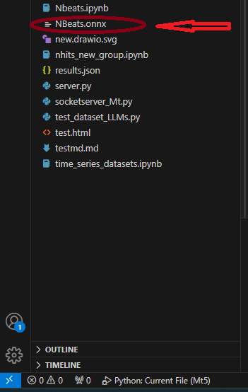
首先,我们定义导出模型所需的 input_sample:input_1=(input_dict,{}) ,别问为什么,照做就是了!然后,我们使用 NBeats 类中的 to_onnx()方法导出到 ONNX,这也需要一个文件路径参数,我们直接导出到根目录,命名为 "NBeats.onnx":best_model.to_onnx(file_path='NBeats.onnx', input_sample=input_1, input_names=input_names, output_names=output_names)。程序运行到这一步后,我们会在当前文件夹的根目录下找到 "NBeats.onnx" 文件:
请注意:
1.因为如果输入参数名称不完整,导出模型时会自动命名,这会造成一定的混乱,让我们不知道哪个才是真正的输入参数,所以我们选择将所有名称都输入到导出函数中,以保证导出模型中输入名称的一致性。
2.在 Dataloader 中,输入数据包括 "encoder_cat"、"encoder_cont "以及编码器和解码器生成的其他多个输入参数,而在推理过程中,我们只需要 "encoder_cont "和 "target_scale "两个输入参数。因此,不要认为匹配输入数据这一步骤是多余的,在某些需要编码器和解码器的模型中,这一步骤是必要的。3.作者在测试过程中使用的环境配置:python-3.10;ONNX 版本-8; pytorch-2.1.1;operators-17.测试转换后的模型
在上一部分中,我们成功地将 torch 模型导出为 ONNX 模型。接下来的重要任务是测试这个模型,看看这个模型的输出结果是否与原始模型相同。这一点非常重要,因为在导出过程中,由于 torch 版本和 onnx 运行时内核的兼容性问题,一些操作符可能会出现偏差。在这种情况下,导出模型时可能需要人工干预。- 首先,导入 ONNX 运行时库:import onnxruntime as ort.
- 加载模型文件 "NBeats.onnx": sess = ort.InferenceSession("NBeats.onnx").
- 通过遍历 sess.get_inputs() 的返回值获取 ONNX 模型的输入名称,这些名称用于匹配输入数据:input_names = [input.name for input in sess.get_inputs()].
- 我们不需要比较所有的输出结果,因此我们只获取输出结果的第一项来比较,看看结果是否相同: output_name = sess.get_outputs()[0].name。
- 要比较结果是否相同,输入必须相同,因此模型输入必须与用于推理的数据一致。但我们需要先将其转换为 Dataloader 格式,并使用 input_names 来匹配输入数据,因为在推理过程中不会加载所有输入数据。首先,使用 TimeSeriesDataSet 类的 from_parameters() 方法将输入数据加载为时间序列数据:input_ds = New_TmSrDt.from_parameters(best_model.dataset_parameters, input_,predict=True)。然后使用 to_dataloader() 类方法将其转换为 Dataloader 类型:input_dl = input_ds.to_dataloader(train=False, batch_size=1, num_workers=0)。
- 匹配输入数据。首先,我们需要获取一批数据并取出第一个元素:input_dict = next(iter(input_dl))[0].然后使用 input_names 中的名称来匹配输入所需的输入数据: input_data = [input_dict[name].numpy() for name in input_names]
- 运行推理: pred_onnx = sess.run([output_name], dict(zip(input_names, input_data))[0]。
- 打印 torch 推理结果和 onnx 推理结果并进行比较。
torch result: tensor([[2062.9109, 2062.6191, 2062.5283, 2062.4814, 2062.3572, 2062.1545, 2061.9824, 2061.9678, 2062.1499, 2062.4380, 2062.6680, 2062.7151, 2062.5823, 2062.3979, 2062.3254, 2062.4460, 2062.7087, 2062.9802, 2063.1643, 2063.2991]])
打印 onnx 推理结果:
onnx result: [[2062.911 2062.6191 2062.5283 2062.4814 2062.3572 2062.1545 2061.9824 2061.9678 2062.15 2062.438 2062.668 2062.715 2062.5823 2062.398 2062.3254 2062.446 2062.7087 2062.9802 2063.1646 2063.299 ]]].
我们可以看到,我们的模型推理结果是一样的。下一步是在 mql5 中配置导出的模型。如图所示:

完整代码:
# Copyright 2021, MetaQuotes Ltd.
# https://www.mql5.com


import lightning.pytorch as pl
import os
from lightning.pytorch.callbacks import EarlyStopping,ModelCheckpoint
import matplotlib.pyplot as plt
import pandas as pd
from pytorch_forecasting import TimeSeriesDataSet,NBeats
from pytorch_forecasting.data import NaNLabelEncoder
from pytorch_forecasting.data.samplers import TimeSynchronizedBatchSampler
from lightning.pytorch.tuner import Tuner
import MetaTrader5 as mt
import warnings
import json

from torch.utils.data import DataLoader
from torch.utils.data.sampler import Sampler,SequentialSampler

class New_TmSrDt(TimeSeriesDataSet):
    '''
    rewrite dataset class
    '''
    def to_dataloader(self, train: bool = True,
                      batch_size: int = 64,
                      batch_sampler: Sampler | str = None,
                      shuffle:bool=False,
                      drop_last:bool=False,
                      **kwargs) -> DataLoader:

        default_kwargs = dict(
            shuffle=shuffle,
            # drop_last=train and len(self) > batch_size,
            drop_last=drop_last, #
            collate_fn=self._collate_fn,
            batch_size=batch_size,
            batch_sampler=batch_sampler,
        )
        default_kwargs.update(kwargs)
        kwargs = default_kwargs
        # print(kwargs['drop_last'])
        if kwargs["batch_sampler"] is not None:
            sampler = kwargs["batch_sampler"]
            if isinstance(sampler, str):
                if sampler == "synchronized":
                    kwargs["batch_sampler"] = TimeSynchronizedBatchSampler(
                        SequentialSampler(self),
                        batch_size=kwargs["batch_size"],
                        shuffle=kwargs["shuffle"],
                        drop_last=kwargs["drop_last"],
                    )
                else:
                    raise ValueError(f"batch_sampler {sampler} unknown - see docstring for valid batch_sampler")
            del kwargs["batch_size"]
            del kwargs["shuffle"]
            del kwargs["drop_last"]

        return DataLoader(self,**kwargs)

def get_data(mt_data_len:int):
    if not mt.initialize():
        print('initialize() failed!')
    else:
        print(mt.version())
        sb=mt.symbols_total()
        rts=None
        if sb > 0:
            rts=mt.copy_rates_from_pos("GOLD_micro",mt.TIMEFRAME_M15,0,mt_data_len)
        mt.shutdown()
        # print(len(rts))
    rts_fm=pd.DataFrame(rts)
    rts_fm['time']=pd.to_datetime(rts_fm['time'], unit='s')

    rts_fm['time_idx']= rts_fm.index%(max_encoder_length+2*max_prediction_length)
    rts_fm['series']=rts_fm.index//(max_encoder_length+2*max_prediction_length)
    return rts_fm


def spilt_data(data:pd.DataFrame,
               t_drop_last:bool,
               t_shuffle:bool,
               v_drop_last:bool,
               v_shuffle:bool):
    training_cutoff = data["time_idx"].max() - max_prediction_length #max:95
    context_length = max_encoder_length
    prediction_length = max_prediction_length
    training = New_TmSrDt(
        data[lambda x: x.time_idx <= training_cutoff],
        time_idx="time_idx",
        target="close",
        categorical_encoders={"series":NaNLabelEncoder().fit(data.series)},
        group_ids=["series"],
        time_varying_unknown_reals=["close"],
        max_encoder_length=context_length,
        # min_encoder_length=max_encoder_length//2,
        max_prediction_length=prediction_length,
        # min_prediction_length=1,

    )

    validation = New_TmSrDt.from_dataset(training,
                                         data,
                                         min_prediction_idx=training_cutoff + 1)

    train_dataloader = training.to_dataloader(train=True,
                                              shuffle=t_shuffle,
                                              drop_last=t_drop_last,
                                              batch_size=batch_size,
                                              num_workers=0,)
    val_dataloader = validation.to_dataloader(train=False,
                                              shuffle=v_shuffle,
                                              drop_last=v_drop_last,
                                              batch_size=batch_size,
                                              num_workers=0)
    return train_dataloader,val_dataloader,training

def get_learning_rate():

    pl.seed_everything(42)
    trainer = pl.Trainer(accelerator="cpu", gradient_clip_val=0.1,logger=False)
    net = NBeats.from_dataset(
        training,
        learning_rate=3e-2,
        weight_decay=1e-2,
        backcast_loss_ratio=0.1,
        optimizer="AdamW",
    )
    res = Tuner(trainer).lr_find(
        net, train_dataloaders=t_loader, val_dataloaders=v_loader, min_lr=1e-5, max_lr=1e-1
    )
    # print(f"suggested learning rate: {res.suggestion()}")
    lr_=res.suggestion()
    return lr_
def train():
    early_stop_callback = EarlyStopping(monitor="val_loss",
                                        min_delta=1e-4,
                                        patience=10,
                                        verbose=True,
                                        mode="min")
    ck_callback=ModelCheckpoint(monitor='val_loss',
                                mode="min",
                                save_top_k=1,
                                filename='{epoch}-{val_loss:.2f}')
    trainer = pl.Trainer(
        max_epochs=ep,
        accelerator="cpu",
        enable_model_summary=True,
        gradient_clip_val=1.0,
        callbacks=[early_stop_callback,ck_callback],
        limit_train_batches=30,
        enable_checkpointing=True,
    )
    net = NBeats.from_dataset(
        training,
        learning_rate=lr,
        log_interval=10,
        log_val_interval=1,
        weight_decay=1e-2,
        backcast_loss_ratio=0.0,
        optimizer="AdamW",
        stack_types=["trend", "seasonality"],
    )
    trainer.fit(
        net,
        train_dataloaders=t_loader,
        val_dataloaders=v_loader,
        # ckpt_path='best'
    )
    return trainer

if __name__=='__main__':
    ep=200
    __train=False
    mt_data_len=80000
    max_encoder_length = 96
    max_prediction_length = 20
    # context_length = max_encoder_length
    # prediction_length = max_prediction_length
    batch_size = 128
    info_file='results.json'
    warnings.filterwarnings("ignore")
    dt=get_data(mt_data_len=mt_data_len)
    if __train:
        # print(dt)
        # dt=get_data(mt_data_len=mt_data_len)
        t_loader,v_loader,training=spilt_data(dt,
                                              t_shuffle=False,t_drop_last=True,
                                              v_shuffle=False,v_drop_last=True)
        lr=get_learning_rate()
        # lr=3e-3
        trainer__=train()
        m_c_back=trainer__.checkpoint_callback
        m_l_back=trainer__.early_stopping_callback
        best_m_p=m_c_back.best_model_path
        best_m_l=m_l_back.best_score.item()

        # print(best_m_p)

        if os.path.exists(info_file):
            with open(info_file,'r+') as f1:
                last=json.load(fp=f1)
                last_best_model=last['last_best_model']
                last_best_score=last['last_best_score']
                if last_best_score > best_m_l:
                    last['last_best_model']=best_m_p
                    last['last_best_score']=best_m_l
                    json.dump(last,fp=f1)
        else:
            with open(info_file,'w') as f2:
                json.dump(dict(last_best_model=best_m_p,last_best_score=best_m_l),fp=f2)

        best_model = NBeats.load_from_checkpoint(best_m_p)
        predictions = best_model.predict(v_loader, trainer_kwargs=dict(accelerator="cpu",logger=False), return_y=True)
        raw_predictions = best_model.predict(v_loader, mode="raw", return_x=True, trainer_kwargs=dict(accelerator="cpu",logger=False))

        for idx in range(10):  # plot 10 examples
            best_model.plot_prediction(raw_predictions.x, raw_predictions.output, idx=idx, add_loss_to_title=True)
        plt.show()
    else:
        with open(info_file) as f:
            best_m_p=json.load(fp=f)['last_best_model']
        print('model path is:',best_m_p)
        best_model = NBeats.load_from_checkpoint(best_m_p)

        # added for input
        best_model.eval()
        t_loader,v_loader,training=spilt_data(dt,
                                t_shuffle=False,t_drop_last=True,
                                v_shuffle=False,v_drop_last=True)

        input_dict = {}
        items = next(iter(v_loader))[0]
        input_names=[]
        for item in items:
            input_dict[item] = items[item][-1:]
            # print("{}:{}".format(item,input_dict[item].shape()))
            input_names.append(item)
# ------------------------eval----------------------------------------------

        offset=1
        dt=dt.iloc[-max_encoder_length-offset:-offset,:]
        last_=dt.iloc[-1]
        # print(len(dt))
        for i in range(1,max_prediction_length+1):
            dt.loc[dt.index[-1]+1]=last_
        dt['series']=0
        # dt['time_idx']=dt.apply(lambda x:x.index,args=1)
        dt['time_idx']=dt.index-dt.index[0]
        input_=dt.loc[:,['close','series','time_idx']]
        predictions = best_model.predict(input_, mode='raw',trainer_kwargs=dict(accelerator="cpu",logger=False),return_x=True)

        output_names=[]
        for out in predictions.output._fields:
            output_names.append(out)
# ----------------------------------------------------------------------------

        input_1=(input_dict,{})
        best_model.to_onnx(file_path='NBeats.onnx',
                           input_sample=input_1,
                           input_names=input_names,
                           output_names=output_names)

        import onnxruntime as ort
        sess = ort.InferenceSession("NBeats.onnx")
        input_names = [input.name for input in sess.get_inputs()]
        # for input in sess.get_inputs():
        #     print(input.name,':',input.shape)
        output_name = sess.get_outputs()[0].name

# ------------------------------------------------------------------------------
        input_ds = New_TmSrDt.from_parameters(best_model.dataset_parameters, input_,predict=True)
        input_dl = input_ds.to_dataloader(train=False, batch_size=1, num_workers=0)
        input_dict = next(iter(input_dl))[0]
        input_data = [input_dict[name].numpy() for name in input_names]
        pred_onnx = sess.run([output_name], dict(zip(input_names, input_data)))
        print("torch result:",predictions.output[0])
        print("onnx result:",pred_onnx[0])
# -------------------------------------------------------------------------------


        best_model.plot_interpretation(predictions.x,predictions.output,idx=0)
        plt.show()
使用 ONNX 模型创建 EA
我们已经完成了模型转换和测试,现在将创建一个名为 onnx.mq5 的专家文件。在 EA 中,我们计划使用 OnTimer() 来管理模型的推理逻辑,并使用 OnTick() 来管理订单逻辑,这样我们就可以设置多久运行一次推理,而不是每次报价时都运行推理,这样会严重占用资源。同样,在本 EA 中,我们不会提供复杂的交易逻辑,只是提供一个演示实例,请不要直接使用本 EA 进行交易!
1.查看 ONNX 模型结构
这一步非常重要,我们需要在 EA 中定义 ONNX 模型的输入和输出,因此需要查看模型结构,确定输入和输出的数量、数据类型和数据维度。要查看 ONNX 模型,可以直接在 mql5 编辑器中打开,然后就能看到模型结构。它还会提供输入和输出的样式,但不可编辑。我们还可以使用 Netron 或 WinML Dashboard 工具,本文中使用的工具是 Netron。
我们在 mql5 集成开发环境中找到模型文件 "NBeats.onnx" 并直接打开它,在下面的注释位置可以找到 "在 Netron 中打开" 选项,点击该按钮,模型文件将自动打开。

或者在集成开发环境的文件资源管理器中使用鼠标右键点击我们的模型文件,你会看到 "在 Netron 中打开" 选项。

如果您没有 Netron 工具,集成开发环境会指导您安装。
模型打开后是这样的:

可以看到,整个界面非常简洁清爽,功能也非常强大。我们甚至可以用它来编辑模型的节点。现在回到主题,我们点击第一个节点,Netron 就会显示模型的相关信息:

可以看到,导出的 NBeats 模型格式为:ONNX v8,pytorch 版本为:pytorch 2.1.1,导出工具为:ai.onnx v17。
有两个输入,第一个是:encoder_cont,维数为:[1,96,1],数据格式为:float32;第二个是:target_scale,维数为:[1,2],数据格式为:float32。
共有五项输出,第一项是:prediction,维度为:[1,20];第二项是:backcast,维度为:[1,96];其他三项可解释的输出是 trend、seasonality,generic 维度为:[1,116]。所有输出数据格式均为 float32。
2.定义模型的输入和输出
我们已经知道了模型的输入和输出格式,而 mql5 中的 onnx 支持的输入和输出格式是数组、矩阵和向量。现在,让我们在 EA 中定义它们。首先,在 OnTimer() 中定义输入,两者都是数组:
- 第一个输入:matrixf in_normf;
- 第二个输入:float in1[1][2];
因为我们需要在 OnTick() 中调用模型的输出结果,所以在 OnTimer() 中定义模型的输出结果是不合理的,它们需要定义为全局变量。模型推理结果和模型加载的句柄也需要定义为全局变量:
- 模型句柄:long handle;
- 第一个推理结果:vectorf y=vector<float>::Zeros(20);
- 第二个推理结果:vectorf backcast=vector<float>::Zeros(96);
- 第三个推理结果:vectorf trend=vector<float>::Zeros(116);
- 第四个推理结果:vectorf seasonality=vector<float>::Zeros(116);
- 第五个推理结果:vectorf generic=vector<float>::Zeros(116);
- 定义预测结果:string pre=NULL;
3.定义推理逻辑
Ⅰ 初始化
首先,在 EA 中将 ONNX 模型作为外部资源导入:#resource "NBeats.onnx" as uchar ExtModel[]。在 OnInit() 函数中初始化定时器:EventSetTimer(300),该值可自行设置。加载模型并获取模型句柄:handle=OnnxCreateFromBuffer(ExtModel,ONNX_DEBUG_LOGS)。如果要查看模型的输入或输出信息,可以添加以下语句:
   long in_ct=OnnxGetInputCount(handle);
   OnnxTypeInfo inf;
   for(int i=0;i<in_ct;i++){

   Print(OnnxGetInputName(handle,i));
   bool re=OnnxGetInputTypeInfo(handle,i,inf);
   //Print("map:",inf.map,"seq:",inf.sequence,"tensor:",inf.tensor,"type:",inf.type);
   Print(re,GetLastError());
   }
Ⅱ 数据处理
我们之前已经定义了模型的输入和输出,接下来我们需要知道这些变量的具体定义,它们是什么样的数据。这就要求我们在 pytorch_forecasting 库中的 timeseries.py 文件中找到它们的定义。本文不会详细解释这个文件,让我们直接揭晓答案吧。
第一个输入:
"encoder_cont "实际上是目标变量的规范化值,当然 pytorch_forecasting 提供了 EncoderNormalizer、GroupNormalizer、MultiNormalizer、NaNLabelEncoder、TorchNormalizer 等不同方法,这些方法在 mql5 中可能难以实现,所以本文直接使用普通的规范化方法。首先定义一个空的 MqlRates:MqlRates rates[],然后用它来复制最近 96 个交易日的收盘值:if(!CopyRates(_Symbol,_Period,0,96,rates)) return,如果复制失败,直接返回。我们还需要定义一个接收该值的矩阵,用于计算均值和方差:matrix in0_m(96,1)。将该报价中的收盘价复制到 in0_m 矩阵: for(int i=0; i<96; i++) in0_m[i][0]= rates[i].close。计算平均数:vector m=in0_m.Mean(0);计算方差:vector s=in0_m.Std(0)。创建一个矩阵 mm 来存储平均值:matrix mm(96,1);创建一个矩阵 ms 来存储方差:matrix ms(96,1)。将均值和方差复制到辅助矩阵中:
    for(int i=0; i<96; i++)
     {
        mm.Row(m,i);
        ms.Row(s,i);
         }
现在我们计算规范化矩阵,首先减去平均值:in0_m-=mm,然后除以标准差:in0_m/=ms,然后将矩阵复制到输入矩阵,并将数据类型转换为浮点数:in_normf.Assign(in0_m)
第二个输入:
"target_scale" 实际上是目标变量的缩放范围,它的第一个值实际上是目标变量的均值:in1[0][0]=m[0],第二个数据是目标变量的方差:in1[0][1]=s[0]
Ⅲ 运行推理
在运行 ONNX 模型推理时,模型结构中显示的输入和输出必须全部定义,一个都不能少,即使一些你不需要的输入也必须作为参数传递给 OnnxRun() 函数,这一点非常重要,否则它肯定会报错。
   if(!OnnxRun(handle,
      ONNX_DEBUG_LOGS | ONNX_NO_CONVERSION,
      in_normf,
      in1,
      y,
      backcast,
      trend,
      seasonality,
      generic))
    {
      Print("OnnxRun failed, error ",GetLastError());
      OnnxRelease(handle);
      return;
      }
4.推理结果
我们做一个简单的假设:如果预测值的平均值大于当前柱形的最高值和最低值的平均值,我们就认为未来将呈上升趋势,并将预设值设为 "买入",否则将预设值设为 "卖出":
   if (y.Mean()>iHigh(_Symbol,_Period,0)/2+iLow(_Symbol,_Period,0)/2)
      pre="buy";
   else
      pre="sell";
5.订单处理逻辑
这部分内容我们已经在《时间序列挖掘的数据标签(第五部分):在 EA 中使用 Socket 进行应用和测试》一文中做了详细介绍,本文不再做详细介绍,我们只需将主要逻辑复制到 OnTick() 中并直接使用即可。需要注意的是,每次执行后,pre 都会被设置为 NULL,在预测过程中,我们会对这两个值进行赋值,这就保证了订单操作过程和预测过程的同步性,不会受到之前预测值的影响。这一步非常重要,否则会造成一些逻辑混乱,以下是完整的订单处理代码:
void OnTick()
  {
//---
   MqlTradeRequest request;
   MqlTradeResult result;
   //int x=SymbolInfoInteger(_Symbol,SYMBOL_FILLING_MODE);

    if (pre!=NULL)
    {
        //Print("The predicted value is:",pre);
        ulong numt=0;
        ulong tik=0;
        bool sod=false;
        ulong tpt=-1;
        ZeroMemory(request);
        numt=PositionsTotal();
        //Print("All tickets: ",numt);
        if (numt>0)
         {  tik=PositionGetTicket(numt-1);
            sod=PositionSelectByTicket(tik);
            tpt=PositionGetInteger(POSITION_TYPE);//ORDER_TYPE_BUY or ORDER_TYPE_SELL
            if (tik==0 || sod==false || tpt==0) return;
            }
        if (pre=="buy")
        {

           if (tpt==POSITION_TYPE_BUY)
               return;

            request.action=TRADE_ACTION_DEAL;
            request.symbol=Symbol();
            request.volume=0.1;
            request.deviation=5;
            request.type_filling=ORDER_FILLING_IOC;
            request.type = ORDER_TYPE_BUY;
            request.price = SymbolInfoDouble(Symbol(), SYMBOL_ASK);
           if(tpt==POSITION_TYPE_SELL)
             {
               request.position=tik;
               Print("Close sell order.");
                    }
           else{

            Print("Open buy order.");
                     }
            OrderSend(request, result);
               }
        else{
           if (tpt==POSITION_TYPE_SELL)
               return;

            request.action = TRADE_ACTION_DEAL;
            request.symbol = Symbol();
            request.volume = 0.1;
            request.type = ORDER_TYPE_SELL;
            request.price = SymbolInfoDouble(Symbol(), SYMBOL_BID);
            request.deviation = 5;
            //request.type_filling=SymbolInfoInteger(_Symbol,SYMBOL_FILLING_MODE);
            request.type_filling=ORDER_FILLING_IOC;
           if(tpt==POSITION_TYPE_BUY)
               {
               request.position=tik;
               Print("Close buy order.");
                    }
           else{

               Print("OPen sell order.");
                    }

            OrderSend(request, result);
              }
        //is_pre=false;
        }
    pre=NULL;

  }
6.回收资源
当 EA 运行时,我们需要关闭计时器并释放 ONNX 模型实例句柄,因此需要在 OnDeinit(const int reason) 函数中添加以下代码:
void OnDeinit(const int reason)
  {
//---
   //— destroy timer
  EventKillTimer();
  //— complete operation
  OnnxRelease(handle);
  }
至此,我们基本上完成了代码编写,然后需要在回测中加载并测试 EA。
请注意:
1.在设置 ONNX 模型的输入和输出时,需要注意数据格式的匹配。
2.我们在这里只使用第一个预测输出值,这并不意味着其他输出值没有价值。在本系列的 "用于时间序列挖掘的数据标签(第四部分):使用标签数据的可解释性分解"一文中,我们介绍了使用其他输出实现的 NBeats 模型的可解释性。我们已经用 python 验证了它们的可视化,本文将不再在 EA 中添加可视化功能。有兴趣的读者可以尝试将其中一个或多个添加到图表中,以实现可视化。
回溯测试
在开始回溯测试之前,有一点需要注意:我们的 ONNX 模型必须与 onnx.mq5 文件放在同一目录下,否则将无法加载模型文件!一切准备就绪,现在打开 mql5 编辑器,点击编译按钮,并生成编译文件。如果编译顺利,按 Ctrl+F5 开始调试模式下的回溯测试。将打开一个新窗口,显示测试过程。我的输出日志:

回溯测试结果:

我们成功了!
完整代码:
//+------------------------------------------------------------------+
//|                                                         onnx.mq5 |
//|                                  Copyright 2023, MetaQuotes Ltd. |
//|                                             https://www.mql5.com |
//+------------------------------------------------------------------+
#property copyright "Copyright 2023, MetaQuotes Ltd."
#property link      "https://www.mql5.com"
#property version   "1.00"

#resource "NBeats.onnx" as uchar ExtModel[]


long handle;
vectorf y=vector<float>::Zeros(20);
vectorf backcast=vector<float>::Zeros(96);
vectorf trend=vector<float>::Zeros(116);
vectorf seasonality=vector<float>::Zeros(116);
vectorf generic=vector<float>::Zeros(116);
//bool is_pre=false;
string pre=NULL;

//+------------------------------------------------------------------+
//| Expert initialization function                                   |
//+------------------------------------------------------------------+
int OnInit()
  {
//---
   EventSetTimer(300);
   handle=OnnxCreateFromBuffer(ExtModel,ONNX_DEBUG_LOGS);
   //— specify the shape of the input data

   long in_ct=OnnxGetInputCount(handle);
   OnnxTypeInfo inf;
   for(int i=0;i<in_ct;i++){

   Print(OnnxGetInputName(handle,i));
   bool re=OnnxGetInputTypeInfo(handle,i,inf);
   //Print("map:",inf.map,"seq:",inf.sequence,"tensor:",inf.tensor,"type:",inf.type);
   Print(re,GetLastError());
   }
   //long in_nm=OnnxGetInputName()


//— return initialization result

//---
   return(INIT_SUCCEEDED);
  }
//+------------------------------------------------------------------+
//| Expert deinitialization function                                 |
//+------------------------------------------------------------------+
void OnDeinit(const int reason)
  {
//---
   //— destroy timer
  EventKillTimer();
  //— complete operation
  OnnxRelease(handle);
  }
//+------------------------------------------------------------------+
//| Expert tick function                                             |
//+------------------------------------------------------------------+
void OnTick()
  {
//---
   MqlTradeRequest request;
   MqlTradeResult result;
   //int x=SymbolInfoInteger(_Symbol,SYMBOL_FILLING_MODE);

    if (pre!=NULL)
    {
        //Print("The predicted value is:",pre);
        ulong numt=0;
        ulong tik=0;
        bool sod=false;
        ulong tpt=-1;
        ZeroMemory(request);
        numt=PositionsTotal();
        //Print("All tickets: ",numt);
        if (numt>0)
         {  tik=PositionGetTicket(numt-1);
            sod=PositionSelectByTicket(tik);
            tpt=PositionGetInteger(POSITION_TYPE);//ORDER_TYPE_BUY or ORDER_TYPE_SELL
            if (tik==0 || sod==false || tpt==0) return;
            }
        if (pre=="buy")
        {

           if (tpt==POSITION_TYPE_BUY)
               return;

            request.action=TRADE_ACTION_DEAL;
            request.symbol=Symbol();
            request.volume=0.1;
            request.deviation=5;
            request.type_filling=ORDER_FILLING_IOC;
            request.type = ORDER_TYPE_BUY;
            request.price = SymbolInfoDouble(Symbol(), SYMBOL_ASK);
           if(tpt==POSITION_TYPE_SELL)
             {
               request.position=tik;
               Print("Close sell order.");
                    }
           else{

            Print("Open buy order.");
                     }
            OrderSend(request, result);
               }
        else{
           if (tpt==POSITION_TYPE_SELL)
               return;

            request.action = TRADE_ACTION_DEAL;
            request.symbol = Symbol();
            request.volume = 0.1;
            request.type = ORDER_TYPE_SELL;
            request.price = SymbolInfoDouble(Symbol(), SYMBOL_BID);
            request.deviation = 5;
            //request.type_filling=SymbolInfoInteger(_Symbol,SYMBOL_FILLING_MODE);
            request.type_filling=ORDER_FILLING_IOC;
           if(tpt==POSITION_TYPE_BUY)
               {
               request.position=tik;
               Print("Close buy order.");
                    }
           else{

               Print("OPen sell order.");
                    }

            OrderSend(request, result);
              }
        //is_pre=false;
        }
    pre=NULL;

  }
//+------------------------------------------------------------------+
void OnTimer()
{
   //float in0[1][96][1];
   matrixf in_normf;
   float in1[1][2];
//— get the last 10 bars
   MqlRates rates[];
   if(!CopyRates(_Symbol,_Period,0,96,rates)) return;
  //— input a set of OHLC vectors


   //double out[1][20];
   matrix in0_m(96,1);
   for(int i=0; i<96; i++)
     {
       in0_m[i][0]= rates[i].close;
       }
   //— normalize the input data
   // matrix x_norm=x;
    vector m=in0_m.Mean(0);
    vector s=in0_m.Std(0);

    in1[0][0]=m[0];
    in1[0][1]=s[0];
    matrix mm(96,1);
    matrix ms(96,1);
   //    //— fill in the normalization matrices
    for(int i=0; i<96; i++)
     {
        mm.Row(m,i);
        ms.Row(s,i);
         }
   //    //— normalize the input data
   in0_m-=mm;
   in0_m/=ms;
   // //— convert normalized input data to float type

   in_normf.Assign(in0_m);
    //— get the output data of the model here, i.e. the price prediction

    //— run the model
   if(!OnnxRun(handle,
      ONNX_DEBUG_LOGS | ONNX_NO_CONVERSION,
      in_normf,
      in1,
      y,
      backcast,
      trend,
      seasonality,
      generic))
    {
      Print("OnnxRun failed, error ",GetLastError());
      OnnxRelease(handle);
      return;
      }
    //— print the output value of the model to the log
   //Print(y);
   //is_pre=true;
   if (y.Mean()>iHigh(_Symbol,_Period,0)/2+iLow(_Symbol,_Period,0)/2)
      pre="buy";
   else
      pre="sell";
}
总结
本文将是本系列的最后一篇文章。在本文中,我们详细介绍了将 torch 模型转换为 ONNX 模型的整个过程,包括如何查找模型的输入和输出、如何定义它们的格式、如何将它们与模型匹配,以及一些数据处理技巧。本文的难点在于如何将具有复杂输入和输出的模型导出为 ONNX 模型。我们希望读者能从中得到启发和收获!当然,我们的测试 EA 还有很大的改进空间。例如,您可以在图表中直观地显示 NBeats 模型输出的趋势和季节性,或利用输出趋势判断订单方向等。
只要你去做,就有无数种可能。文章中的例子只是一个最简单的例子,但核心内容相对完整。您可以自由扩展和使用它,但请注意不要随意将此 EA 用于实际交易!从制作数据集到训练不同的时间序列预测模型,再到如何在回测中使用这些模型,本系列文章提供了各种相对完整的解决方案。即使是初学者也能一步步完成整个过程,并将其应用到实践中,因此本系列可以圆满结束!
感谢您的阅读,希望您有所收获,祝您愉快!
本文由MetaQuotes Ltd译自英文
原文地址: https://www.mql5.com/en/articles/13919
 使用 Python 和 MetaTrader5 python 软件包及 ONNX 模型文件进行深度学习预测和排序