
数据科学和机器学习(第 16 部分):全新面貌的决策树

快速回顾
在本系列文章中,我撰写了一篇关于决策树的文章,解释了决策树的全部内容,并且我们还构建了一个算法来帮助我们对天气数据进行分类。不过,文章中提供的代码和解释不够简洁;随着我不断收到要求提供更佳方式来构建决策树的请求,我相信撰写第二篇文章,并为决策树提供更好的代码也许会更好。厘清决策树将令人们更容易理解即将发表的文章中所采用的随机森林算法。
什么是决策树?
决策树是一种类似流程图的树形结构,其中每个内部节点代表一个属性(或特征)的测试,每条分支代表测试的结果,每个叶节点代表一个类标签或连续值。决策树中最顶层的节点被称为“根”,叶子是结果或预测。
什么是节点?
在决策树中,节点是一个基本组件,表示基于特定特征或属性的决策点。决策树中有两种主要类型的节点:内部节点和叶节点。
内部节点- 内部节点是树中的一个决策点,其为针对具体特征执行的测试。该测试依赖于特定条件,诸如特征值是否大于阈值、或是否属于特定类别。
- 内部节点具有指向子节点的分支(边)。测试的成果决定了要遵循的分支。
- 内部节点是两个左右子节点,是中心树节点内的节点。
- 叶节点标记树中的一个终端点,它在该处做出最终决策或预测。它表示分类任务中的类标签、或回归任务中的预测值。
- 叶节点没有外延分支;它们是决策过程的终点。
- 我们在编码时作为双精度变量。
class Node
{
  public:
    // for decision node

    uint feature_index;
    double threshold;
    double info_gain;

    // for leaf node

    double leaf_value;

    Node *left_child;  //left child Node
    Node *right_child; //right child Node

    Node() : left_child(NULL), right_child(NULL) {} // default constructor

    Node(uint feature_index_, double threshold_=NULL, Node *left_=NULL, Node *right_=NULL, double info_gain_=NULL, double value_=NULL)
        : left_child(left_), right_child(right_)
    {
        this.feature_index = feature_index_;
        this.threshold = threshold_;
        this.info_gain = info_gain_;
        this.value = value_;
    }

   void Print()
    {
      printf("feature_index: %d \nthreshold: %f \ninfo_gain: %f \nleaf_value: %f",feature_index,threshold, info_gain, value);
    }
};
与我们在本系列中从头开始编写的一些 ML 算法不同,决策树的编码可能很棘手,有时还会令人困惑,因为它需要递归类和函数才能很好地实现,根据我的经验,使用 Python 以外的语言编写这些内容可能很困难。
节点的组件:
决策树中的节点通常包含以下信息:
01. 测试条件
内部节点拥有基于具体特征和阈值、或类别的测试条件。该条件判定如何将数据拆分为子节点。
Node *build_tree(matrix &data, uint curr_depth=0);
02. 特征和阈值
指示在节点上正在测试哪个特征,以及用于拆分的阈值或类别。
uint feature_index;
double threshold;
03. 类标签或数值
叶节点存储预测的类标签(用于分类)、或数值(用于回归)
double leaf_value; 04. 子节点
内部节点拥有对应于测试条件的不同结果的子节点。每个子节点都表示满足条件的数据子集。
Node *left_child;  //left child Node
Node *right_child; //right child Node
例如:
研究一棵简单的决策树,基于水果的颜色把水果分类为苹果或橙子;
[Node]
特征:颜色
测试条件:颜色是红色的吗?
如果为 True,则转至左边子叶;如果为 False,则转至右边子叶
[Leaf Node - Apple]
-类标签:苹果
[Leaf Node - Orange]
-类标签:橙子
决策树的类型:
CART(分类和回归树):用于分类和回归任务。数据拆分基于基尼(Gini)杂质进行分类,根据均方误差进行回归。
ID3(迭代二分法器 3):主要用于分类任务。采用熵和信息增益的概念来做出决策。
C4.5:ID3 的改进版本,C4.5 用于分类。它采用增益比率来定位具有更多级别的属性偏向。
由于我们将寻求使用决策树进行分类目的,因此我们将寻求构建的 ID3 算法,以信息增益、杂质计算、和分类特征为特征:
ID3(迭代二分法器 3)
ID3 使用信息增益来决定在每个内部节点上拆分哪个特征。信息增益衡量的是数据集拆分后熵或不确定性的减少。double CDecisionTree::information_gain(vector &parent, vector &left_child, vector &right_child) { double weight_left = left_child.Size() / (double)parent.Size(), weight_right = right_child.Size() / (double)parent.Size(); double gain =0; switch(m_mode) { case MODE_GINI: gain = gini_index(parent) - ( (weight_left*gini_index(left_child)) + (weight_right*gini_index(right_child)) ); break; case MODE_ENTROPY: gain = entropy(parent) - ( (weight_left*entropy(left_child)) + (weight_right*entropy(right_child)) ); break; } return gain; }
熵是数据集中不确定性或无序性的度量。在 ID3 中,该算法尝试通过选择特征拆分来减少熵,从而产生拥有更多同质类标签的子集。
double CDecisionTree::entropy(vector &y)
 {
   vector class_labels = matrix_utils.Unique_count(y);

   vector p_cls = class_labels / double(y.Size());

   vector entropy = (-1 * p_cls) * log2(p_cls);

  return entropy.Sum();
 }
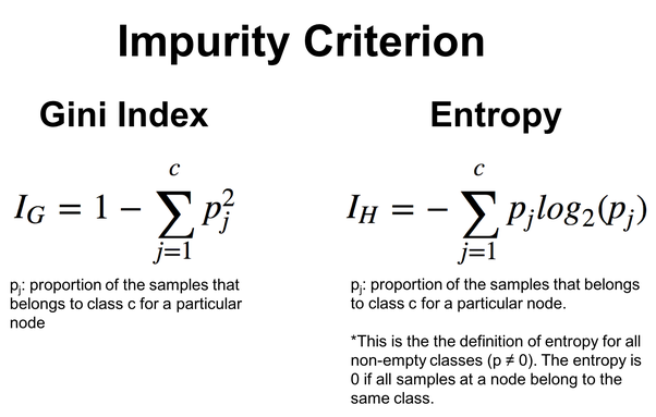
为了提供更大的灵活性,可以在熵和基尼指数之间进行选择,基尼指数也是决策树中经常使用的函数,其工作与熵函数相同。它们都评估数据集中的杂质或无序。
double CDecisionTree::gini_index(vector &y)
 {
   vector unique = matrix_utils.Unique_count(y);

   vector probabilities = unique / (double)y.Size();

   return 1.0 - MathPow(probabilities, 2).Sum();
 }
下图给出公式:
ID3 特别适用于分类特征,且特征和阈值的选择基于分类拆分的熵减少。我们将在下面的决策树算法中看到这一点。
决策树算法
01. 拆分准则
为了分类,标准拆分准则是基尼杂质和熵,而均方误差通常用于回归。我们来深入研究决策树算法的拆分函数,该函数从结构开始,为的是保留正在拆分数据的信息。
//A struct containing splitted data information
struct split_info
  {
   uint feature_index;
   double threshold;
   matrix dataset_left,
          dataset_right;
   double info_gain;
  };
使用阈值,我们将数值小于阈值的特征拆分到矩阵 dataset_left,同时将其余的特征保留到矩阵 dataset_right。最后,返回 split_info 结构实例。
split_info CDecisionTree::split_data(const matrix &data, uint feature_index, double threshold=0.5)
 {
   int left_size=0, right_size =0;
   vector row = {};

   split_info split;

   ulong cols = data.Cols();

   split.dataset_left.Resize(0, cols);
   split.dataset_right.Resize(0, cols);

    for (ulong i=0; i<data.Rows(); i++)
     {
       row = data.Row(i);

       if (row[feature_index] <= threshold)
        {
          left_size++;
          split.dataset_left.Resize(left_size, cols);
          split.dataset_left.Row(row, left_size-1);
        }
       else
        {
         right_size++;
         split.dataset_right.Resize(right_size, cols);
         split.dataset_right.Row(row, right_size-1);
        }
     }
   return split;
 }
从众多拆分当中,算法需要找出最好的拆分,即拥有最大信息增益的那个。
split_info CDecisionTree::get_best_split(matrix &data, uint num_features)
  {

   double max_info_gain = -DBL_MAX;
   vector feature_values = {};
   vector left_v={}, right_v={}, y_v={};

//---

   split_info best_split;
   split_info split;

   for (uint i=0; i<num_features; i++)
     {
       feature_values = data.Col(i);
       vector possible_thresholds = matrix_utils.Unique(feature_values); //Find unique values in the feature, representing possible thresholds for splitting.

         for (uint j=0; j<possible_thresholds.Size(); j++)
            {
              split = this.split_data(data, i, possible_thresholds[j]);

              if (split.dataset_left.Rows()>0 && split.dataset_right.Rows() > 0)
                {
                  y_v = data.Col(data.Cols()-1);
                  right_v = split.dataset_right.Col(split.dataset_right.Cols()-1);
                  left_v = split.dataset_left.Col(split.dataset_left.Cols()-1);

                  double curr_info_gain = this.information_gain(y_v, left_v, right_v);

                  if (curr_info_gain > max_info_gain) // Check if the current information gain is greater than the maximum observed so far.
                    {
                      #ifdef DEBUG_MODE
                        printf("split left: [%dx%d] split right: [%dx%d] curr_info_gain: %f max_info_gain: %f",split.dataset_left.Rows(),split.dataset_left.Cols(),split.dataset_right.Rows(),split.dataset_right.Cols(),curr_info_gain,max_info_gain);
                      #endif

                      best_split.feature_index = i;
                      best_split.threshold = possible_thresholds[j];
                      best_split.dataset_left = split.dataset_left;
                      best_split.dataset_right = split.dataset_right;
                      best_split.info_gain = curr_info_gain;

                      max_info_gain = curr_info_gain;
                    }
                }
            }
     }

    return best_split;
  }
该函数搜索整体特征和可能的阈值,以便找到最大化信息增益的最佳拆分。结果是一个 split_info 结构,其中包含有关与最佳拆分关联的特征、阈值和子集的信息。
02. 构造树
决策树是基于特征递归拆分数据集来构建的,直到满足停止条件(例如,达到一定深度、或最小样本)。
Node *CDecisionTree::build_tree(matrix &data, uint curr_depth=0)
 {
    matrix X;
    vector Y;

    matrix_utils.XandYSplitMatrices(data,X,Y); //Split the input matrix into feature matrix X and target vector Y.

    ulong samples = X.Rows(), features = X.Cols(); //Get the number of samples and features in the dataset.

    Node *node= NULL; // Initialize node pointer

    if (samples >= m_min_samples_split && curr_depth<=m_max_depth)
      {
         split_info best_split = this.get_best_split(data, (uint)features);

         #ifdef DEBUG_MODE
          Print("best_split left: [",best_split.dataset_left.Rows(),"x",best_split.dataset_left.Cols(),"]\nbest_split right: [",best_split.dataset_right.Rows(),"x",best_split.dataset_right.Cols(),"]\nfeature_index: ",best_split.feature_index,"\nInfo gain: ",best_split.info_gain,"\nThreshold: ",best_split.threshold);
         #endif

         if (best_split.info_gain > 0)
           {
             Node *left_child = this.build_tree(best_split.dataset_left, curr_depth+1);
             Node *right_child = this.build_tree(best_split.dataset_right, curr_depth+1);

             node = new Node(best_split.feature_index,best_split.threshold,left_child,right_child,best_split.info_gain);
             return node;
           }
      }

     node = new Node();
     node.leaf_value = this.calculate_leaf_value(Y);

     return node;
 }
if (best_split.info_gain > 0):
上面的代码行检查是否获得了信息。
在此模块内:
Node *left_child = this.build_tree(best_split.dataset_left, curr_depth+1);
递归构建左侧子节点。
Node *right_child = this.build_tree(best_split.dataset_right, curr_depth+1);
递归构建右侧子节点。
node = new Node(best_split.feature_index, best_split.threshold, left_child, right_child, best_split.info_gain);
依据最佳拆分中的信息创建一个决策节点。
node = new Node(); 如果不需要进一步拆分,创建新的叶节点。
node.value = this.calculate_leaf_value(Y); 调用 calculate_leaf_value 函数设置叶节点的数值。
return node; 返回代表当前拆分或叶的节点。
为了令函数便捷及用户友好,可以将 build_tree 函数保留在 fit 函数内部,fit 函数通常在 Python 机器学习模块当中用到。
void CDecisionTree::fit(matrix &x, vector &y)
 {
   matrix data = matrix_utils.concatenate(x, y, 1);

   this.root = this.build_tree(data);
 }
对模型的训练和测试进行预测
vector CDecisionTree::predict(matrix &x)
 {
    vector ret(x.Rows());

    for (ulong i=0; i<x.Rows(); i++)
       ret[i] = this.predict(x.Row(i));

   return ret;
 }
实时预测
double CDecisionTree::predict(vector &x)
 {
   return this.make_predictions(x, this.root);
 }
make_predictions 函数是完成所有辛苦工作的所在:
double CDecisionTree::make_predictions(vector &x, const Node &tree)
 {
    if (tree.leaf_value != NULL) // This is a leaf leaf_value
      return tree.leaf_value;

    double feature_value = x[tree.feature_index];
    double pred = 0;

    #ifdef DEBUG_MODE
      printf("Tree.threshold %f tree.feature_index %d leaf_value %f",tree.threshold,tree.feature_index,tree.leaf_value);
    #endif

    if (feature_value <= tree.threshold)
      {
       pred = this.make_predictions(x, tree.left_child);
      }
    else
     {
       pred = this.make_predictions(x, tree.right_child);
     }

   return pred;
 }
有关该函数的更多详情:
if (feature_value <= tree.threshold): 在此模块内:
递归调用左侧子节点的 make_predictions。
pred = this.make_predictions(x, *tree.left_child); 否则,如果特征值大于阈值:
递归调用右侧子节点的 make_predictions 函数。
pred = this.make_predictions(x, *tree.right_child); return pred; 返回预测。
叶值计算
以下函数计算叶值:
double CDecisionTree::calculate_leaf_value(vector &Y)
 {
   vector uniques = matrix_utils.Unique_count(Y);
   vector classes = matrix_utils.Unique(Y);

   return classes[uniques.ArgMax()];
 }
该函数从 Y 返回计数最高的元素,从而有效地查找列表中最常见的元素。
将其全部封装在 CDecisionTree 类当中
enum mode {MODE_ENTROPY, MODE_GINI};

class CDecisionTree
  {
CMatrixutils   matrix_utils;

protected:

   Node *build_tree(matrix &data, uint curr_depth=0);
   double  calculate_leaf_value(vector &Y);

//---

   uint m_max_depth;
   uint m_min_samples_split;

   mode m_mode;

   double  gini_index(vector &y);
   double  entropy(vector &y);
   double  information_gain(vector &parent, vector &left_child, vector &right_child);


   split_info  get_best_split(matrix &data, uint num_features);
   split_info  split_data(const matrix &data, uint feature_index, double threshold=0.5);

   double make_predictions(vector &x, const Node &tree);
   void delete_tree(Node* node);

public:
                     Node *root;

                     CDecisionTree(uint min_samples_split=2, uint max_depth=2, mode mode_=MODE_GINI);
                    ~CDecisionTree(void);

                     void fit(matrix &x, vector &y);
                     void print_tree(Node *tree, string indent=" ",string padl="");
                     double predict(vector &x);
                     vector predict(matrix &x);
  };
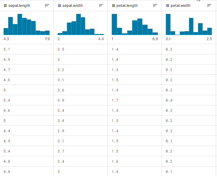
这一点已有所展示,我们来观察一切是如何运作的,如何构建树,以及如何用它来预测训练和测试,更不必提在实时交易期间了。我们将使用最流行的 iris-CSV 数据集来测试它是否有效。
假设我们将在每次 EA 初始化时训练决策树模型,首先从 CSV 文件加载训练数据:
int OnInit()
  {
  matrix dataset = matrix_utils.ReadCsv("iris.csv"); //loading iris-data

  decision_tree = new CDecisionTree(3,3, MODE_GINI); //Initializing the decision tree

  matrix x; vector y;
  matrix_utils.XandYSplitMatrices(dataset,x,y); //split the data into x and y matrix and vector respectively


  decision_tree.fit(x, y);  //Building the tree
  decision_tree.print_tree(decision_tree.root); //Printing the tree

  vector preds = decision_tree.predict(x); //making the predictions on a training data

  Print("Train Acc = ",metrics.confusion_matrix(y, preds)); //Measuring the accuracy

   return(INIT_SUCCEEDED);
  }
这是打印时数据集矩阵的外观。最后一列已编码。一(1)代表 Setosa,二(2)代表 Versicolor,三(3)代表 Virginica
Print("iris-csv\n",dataset);
MS      0       08:54:40.958    DecisionTree Test (EURUSD,H1)   iris-csv
PH      0       08:54:40.958    DecisionTree Test (EURUSD,H1)   [[5.1,3.5,1.4,0.2,1]
CO      0       08:54:40.958    DecisionTree Test (EURUSD,H1)    [4.9,3,1.4,0.2,1]
...
...

NS      0       08:54:40.959    DecisionTree Test (EURUSD,H1)    [5.6,2.7,4.2,1.3,2]
JK      0       08:54:40.959    DecisionTree Test (EURUSD,H1)    [5.7,3,4.2,1.2,2]
...
...

NQ      0       08:54:40.959    DecisionTree Test (EURUSD,H1)    [6.2,3.4,5.4,2.3,3]
PD      0       08:54:40.959    DecisionTree Test (EURUSD,H1)    [5.9,3,5.1,1.8,3]]
打印树
如果您查看代码,您也许已注意到函数 print_tree,它以树根作为其参数之一。该函数尝试打印树的整体外观;仔细查看如下。
void CDecisionTree::print_tree(Node *tree, string indent=" ",string padl="")
  {
     if (tree.leaf_value != NULL)
        Print((padl+indent+": "),tree.leaf_value);
     else //if we havent' reached the leaf node keep printing child trees
       {
         padl += " ";

         Print((padl+indent)+": X_",tree.feature_index, "<=", tree.threshold, "?", tree.info_gain);

         print_tree(tree.left_child, "left","--->"+padl);

         print_tree(tree.right_child, "right","--->"+padl);
       }
  }
有关该函数的更多详情:
节点结构:
该函数假定 Node 类表示决策树。每个节点可以是决策节点,也可以是叶节点。决策节点具有 feature_index、阈值、和一个 leaf_value info_gain 指示特征、阈值、信息增益、及叶数值。
打印决策节点:
如果当前节点不是叶节点(即 tree.leaf_value 为 NULL),则打印有关决策节点的信息。它打印拆分的条件,诸如 "X_2 <= 1.9 ?0.33",以及缩进级别。
打印叶节点:
如果当前节点是叶节点(即 tree.leaf_value 非 NULL),则它将打印叶值,以及缩进级别。例如,"left: 0.33"。
递归:
然后,该函数递归调用自身当前 Node 的左子级和右子级。padl 参数指定打印输出时的缩进,令树结构更具可读性。
由 print_tree 输出的在 OnInit 函数内构建的决策树:
CR      0       09:26:39.990    DecisionTree Test (EURUSD,H1)     : X_2<=1.9?0.3333333333333334
HO      0       09:26:39.990    DecisionTree Test (EURUSD,H1)   ---> left: 1.0
RH      0       09:26:39.990    DecisionTree Test (EURUSD,H1)   --->  right: X_3<=1.7?0.38969404186795487
HP      0       09:26:39.990    DecisionTree Test (EURUSD,H1)   --->--->   left: X_2<=4.9?0.08239026063100136
KO      0       09:26:39.990    DecisionTree Test (EURUSD,H1)   --->--->--->    left: X_3<=1.6?0.04079861111111116
DH      0       09:26:39.990    DecisionTree Test (EURUSD,H1)   --->--->--->--->    left: 2.0
HM      0       09:26:39.990    DecisionTree Test (EURUSD,H1)   --->--->--->--->    right: 3.0
HS      0       09:26:39.990    DecisionTree Test (EURUSD,H1)   --->--->--->    right: X_3<=1.5?0.2222222222222222
IH      0       09:26:39.990    DecisionTree Test (EURUSD,H1)   --->--->--->--->    left: 3.0
QM      0       09:26:39.990    DecisionTree Test (EURUSD,H1)   --->--->--->--->    right: 2.0
KP      0       09:26:39.990    DecisionTree Test (EURUSD,H1)   --->--->   right: X_2<=4.8?0.013547574039067499
PH      0       09:26:39.990    DecisionTree Test (EURUSD,H1)   --->--->--->    left: X_0<=5.9?0.4444444444444444
PE      0       09:26:39.990    DecisionTree Test (EURUSD,H1)   --->--->--->--->    left: 2.0
DP      0       09:26:39.990    DecisionTree Test (EURUSD,H1)   --->--->--->--->    right: 3.0
EE      0       09:26:39.990    DecisionTree Test (EURUSD,H1)   --->--->--->   right: 3.0
令人 印象 深刻。
以下是我们训练的模型准确性:
  vector preds = decision_tree.predict(x); //making the predictions on a training data

  Print("Train Acc = ",metrics.confusion_matrix(y, preds)); //Measuring the accuracy
输出:
PM      0       09:26:39.990    DecisionTree Test (EURUSD,H1)   Confusion Matrix
CE      0       09:26:39.990    DecisionTree Test (EURUSD,H1)   [[50,0,0]
HR      0       09:26:39.990    DecisionTree Test (EURUSD,H1)    [0,50,0]
ND      0       09:26:39.990    DecisionTree Test (EURUSD,H1)    [0,1,49]]
GS      0       09:26:39.990    DecisionTree Test (EURUSD,H1)
KF      0       09:26:39.990    DecisionTree Test (EURUSD,H1)   Classification Report
IR      0       09:26:39.990    DecisionTree Test (EURUSD,H1)
MD      0       09:26:39.990    DecisionTree Test (EURUSD,H1)   _    Precision  Recall  Specificity  F1 score  Support
EQ      0       09:26:39.990    DecisionTree Test (EURUSD,H1)   1.0    50.00     50.00     100.00       50.00     50.0
HR      0       09:26:39.990    DecisionTree Test (EURUSD,H1)   2.0    51.00     50.00     100.00       50.50     50.0
PO      0       09:26:39.990    DecisionTree Test (EURUSD,H1)   3.0    49.00     50.00     100.00       49.49     50.0
EH      0       09:26:39.990    DecisionTree Test (EURUSD,H1)
PR      0       09:26:39.990    DecisionTree Test (EURUSD,H1)   Accuracy                                   0.99
HQ      0       09:26:39.990    DecisionTree Test (EURUSD,H1)   Average   50.00    50.00    100.00      50.00    150.0
DJ      0       09:26:39.990    DecisionTree Test (EURUSD,H1)   W Avg     50.00    50.00    100.00      50.00    150.0
LG      0       09:26:39.990    DecisionTree Test (EURUSD,H1)   Train Acc = 0.993
我们达成了 99.3% 的准确率,表明我们的决策树已成功实现。这种准确性与您在处理简单数据集问题时对 Scikit-Learn 模型的期望一致。
我们继续进行深入训练,并在样本之外的数据上测试模型。
  matrix train_x, test_x;
  vector train_y, test_y;

  matrix_utils.TrainTestSplitMatrices(dataset, train_x, train_y, test_x, test_y, 0.8, 42); //split the data into training and testing samples


  decision_tree.fit(train_x, train_y);  //Building the tree
  decision_tree.print_tree(decision_tree.root); //Printing the tree

  vector preds = decision_tree.predict(train_x); //making the predictions on a training data

  Print("Train Acc = ",metrics.confusion_matrix(train_y, preds)); //Measuring the accuracy

//---

  preds = decision_tree.predict(test_x); //making the predictions on a test data

  Print("Test Acc = ",metrics.confusion_matrix(test_y, preds)); //Measuring the accuracy
输出:
QD      0       14:56:03.860    DecisionTree Test (EURUSD,H1)     : X_2<=1.7?0.34125
LL      0       14:56:03.860    DecisionTree Test (EURUSD,H1)   ---> left: 1.0
QK      0       14:56:03.860    DecisionTree Test (EURUSD,H1)   --->  right: X_3<=1.6?0.42857142857142855
GS      0       14:56:03.860    DecisionTree Test (EURUSD,H1)   --->--->   left: X_2<=4.9?0.09693877551020412
IL      0       14:56:03.860    DecisionTree Test (EURUSD,H1)   --->--->--->   left: 2.0
MD      0       14:56:03.860    DecisionTree Test (EURUSD,H1)   --->--->--->    right: X_3<=1.5?0.375
IS      0       14:56:03.860    DecisionTree Test (EURUSD,H1)   --->--->--->--->    left: 3.0
QR      0       14:56:03.860    DecisionTree Test (EURUSD,H1)   --->--->--->--->    right: 2.0
RH      0       14:56:03.860    DecisionTree Test (EURUSD,H1)   --->--->  right: 3.0
HP      0       14:56:03.860    DecisionTree Test (EURUSD,H1)   Confusion Matrix
FG      0       14:56:03.860    DecisionTree Test (EURUSD,H1)   [[42,0,0]
EO      0       14:56:03.860    DecisionTree Test (EURUSD,H1)    [0,39,0]
HK      0       14:56:03.860    DecisionTree Test (EURUSD,H1)    [0,0,39]]
OL      0       14:56:03.860    DecisionTree Test (EURUSD,H1)
KE      0       14:56:03.860    DecisionTree Test (EURUSD,H1)   Classification Report
QO      0       14:56:03.860    DecisionTree Test (EURUSD,H1)
MQ      0       14:56:03.860    DecisionTree Test (EURUSD,H1)   _    Precision  Recall  Specificity  F1 score  Support
OQ      0       14:56:03.860    DecisionTree Test (EURUSD,H1)   1.0    42.00     42.00     78.00       42.00     42.0
ML      0       14:56:03.860    DecisionTree Test (EURUSD,H1)   3.0    39.00     39.00     81.00       39.00     39.0
HK      0       14:56:03.860    DecisionTree Test (EURUSD,H1)   2.0    39.00     39.00     81.00       39.00     39.0
OE      0       14:56:03.860    DecisionTree Test (EURUSD,H1)
EO      0       14:56:03.860    DecisionTree Test (EURUSD,H1)   Accuracy                                   1.00
CG      0       14:56:03.860    DecisionTree Test (EURUSD,H1)   Average   40.00    40.00    80.00      40.00    120.0
LF      0       14:56:03.860    DecisionTree Test (EURUSD,H1)   W Avg     40.05    40.05    79.95      40.05    120.0
PR      0       14:56:03.860    DecisionTree Test (EURUSD,H1)   Train Acc = 1.0
CD      0       14:56:03.861    DecisionTree Test (EURUSD,H1)   Confusion Matrix
FO      0       14:56:03.861    DecisionTree Test (EURUSD,H1)   [[9,2,0]
RK      0       14:56:03.861    DecisionTree Test (EURUSD,H1)    [1,10,0]
CL      0       14:56:03.861    DecisionTree Test (EURUSD,H1)    [2,0,6]]
HK      0       14:56:03.861    DecisionTree Test (EURUSD,H1)
DQ      0       14:56:03.861    DecisionTree Test (EURUSD,H1)   Classification Report
JJ      0       14:56:03.861    DecisionTree Test (EURUSD,H1)
FM      0       14:56:03.861    DecisionTree Test (EURUSD,H1)   _    Precision  Recall  Specificity  F1 score  Support
QM      0       14:56:03.861    DecisionTree Test (EURUSD,H1)   2.0    12.00     11.00     19.00       11.48     11.0
PH      0       14:56:03.861    DecisionTree Test (EURUSD,H1)   3.0    12.00     11.00     19.00       11.48     11.0
KD      0       14:56:03.861    DecisionTree Test (EURUSD,H1)   1.0    6.00     8.00     22.00       6.86     8.0
PP      0       14:56:03.861    DecisionTree Test (EURUSD,H1)
LJ      0       14:56:03.861    DecisionTree Test (EURUSD,H1)   Accuracy                                   0.83
NJ      0       14:56:03.861    DecisionTree Test (EURUSD,H1)   Average   10.00    10.00    20.00      9.94    30.0
JR      0       14:56:03.861    DecisionTree Test (EURUSD,H1)   W Avg     10.40    10.20    19.80      10.25    30.0
HP      0       14:56:03.861    DecisionTree Test (EURUSD,H1)   Test Acc = 0.833
该模型在训练数据上的准确率为 100%,而在样本之外数据上的准确率为 83%。
交易中的决策树 AI
如果我们不使用决策树模型来探索交易方面,那么所有这些都毫无意义。为了在交易中使用此模型,我们要明确一个我们想要解决的问题。
要解决的问题:
我们想使用决策树 AI 模型对当前柱线进行预测,从而告诉我们市场可能的发展方向,无论是上涨亦或下跌。
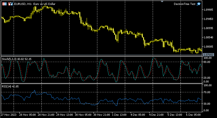
与任何模型一样,我们希望为模型提供一个学习数据集;假设我们决定使用振荡器类型的两个指标,RSI 指标和随机振荡器;基本上,我们希望模型能够理解这两个指标之间的形态,以及它如何影响当前柱线的价格走势。
数据结构:
出于训练测试目的,一旦数据收集完毕,数据就会存储在下面的结构之中。这同样适用于实时预测数据。
struct data{
   vector stoch_buff,
          signal_buff,
          rsi_buff,
          target;
} data_struct;
收集数据、训练、和测试决策树
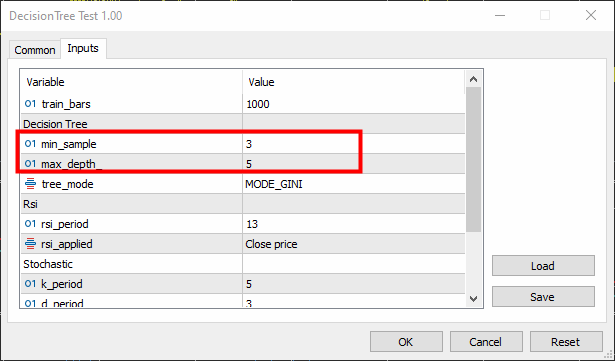
void TrainTree()
 {
  matrix dataset(train_bars, 4);
  vector v;

//--- Collecting indicator buffers

  data_struct.rsi_buff.CopyIndicatorBuffer(rsi_handle, 0, 1, train_bars);
  data_struct.stoch_buff.CopyIndicatorBuffer(stoch_handle, 0, 1, train_bars);
  data_struct.signal_buff.CopyIndicatorBuffer(stoch_handle, 1, 1, train_bars);

//--- Preparing the target variable

  MqlRates rates[];
  ArraySetAsSeries(rates, true);
  int size = CopyRates(Symbol(), PERIOD_CURRENT, 1,train_bars, rates);

  data_struct.target.Resize(size); //Resize the target vector

  for (int i=0; i<size; i++)
    {
      if (rates[i].close > rates[i].open)
        data_struct.target[i] = 1;
      else
        data_struct.target[i] = -1;
    }

  dataset.Col(data_struct.rsi_buff, 0);
  dataset.Col(data_struct.stoch_buff, 1);
  dataset.Col(data_struct.signal_buff, 2);
  dataset.Col(data_struct.target, 3);

  decision_tree = new CDecisionTree(min_sample,max_depth_, tree_mode); //Initializing the decision tree


  matrix train_x, test_x;
  vector train_y, test_y;

  matrix_utils.TrainTestSplitMatrices(dataset, train_x, train_y, test_x, test_y, 0.8, 42); //split the data into training and testing samples


  decision_tree.fit(train_x, train_y);  //Building the tree
  decision_tree.print_tree(decision_tree.root); //Printing the tree

  vector preds = decision_tree.predict(train_x); //making the predictions on a training data

  Print("Train Acc = ",metrics.confusion_matrix(train_y, preds)); //Measuring the accuracy

//---

  preds = decision_tree.predict(test_x); //making the predictions on a test data

  Print("Test Acc = ",metrics.confusion_matrix(test_y, preds)); //Measuring the accuracy
 }
Min-sample 设置为 3,而 max-depth 设置为 5。
输出:
KR      0       16:26:53.028    DecisionTree Test (EURUSD,H1)     : X_0<=65.88930872549261?0.0058610536710859695
CN      0       16:26:53.028    DecisionTree Test (EURUSD,H1)   --->  left: X_0<=29.19882857713344?0.003187469522387243
FK      0       16:26:53.028    DecisionTree Test (EURUSD,H1)   --->--->   left: X_1<=26.851851851853503?0.030198175526895188
RI      0       16:26:53.028    DecisionTree Test (EURUSD,H1)   --->--->--->    left: X_2<=7.319205739522295?0.040050858232676456
KG      0       16:26:53.028    DecisionTree Test (EURUSD,H1)   --->--->--->--->     left: X_0<=23.08345903222593?0.04347468770545693
JF      0       16:26:53.028    DecisionTree Test (EURUSD,H1)   --->--->--->--->--->      left: X_0<=21.6795921184317?0.09375
PF      0       16:26:53.028    DecisionTree Test (EURUSD,H1)   --->--->--->--->--->--->      left: -1.0
ER      0       16:26:53.028    DecisionTree Test (EURUSD,H1)   --->--->--->--->--->--->      right: -1.0
QF      0       16:26:53.028    DecisionTree Test (EURUSD,H1)   --->--->--->--->--->      right: X_2<=3.223853479489069?0.09876543209876543
LH      0       16:26:53.028    DecisionTree Test (EURUSD,H1)   --->--->--->--->--->--->      left: -1.0
FJ      0       16:26:53.028    DecisionTree Test (EURUSD,H1)   --->--->--->--->--->--->      right: 1.0
MM      0       16:26:53.028    DecisionTree Test (EURUSD,H1)   --->--->--->--->    right: -1.0
MG      0       16:26:53.028    DecisionTree Test (EURUSD,H1)   --->--->--->   right: 1.0
HH      0       16:26:53.028    DecisionTree Test (EURUSD,H1)   --->--->   right: X_0<=65.4606831930956?0.0030639039663222234
JR      0       16:26:53.028    DecisionTree Test (EURUSD,H1)   --->--->--->    left: X_0<=31.628407983040333?0.00271101025966336
PS      0       16:26:53.028    DecisionTree Test (EURUSD,H1)   --->--->--->--->     left: X_0<=31.20436037455599?0.0944903581267218
DO      0       16:26:53.028    DecisionTree Test (EURUSD,H1)   --->--->--->--->--->      left: X_2<=14.629981942657205?0.11111111111111116
EO      0       16:26:53.028    DecisionTree Test (EURUSD,H1)   --->--->--->--->--->--->      left: 1.0
IG      0       16:26:53.028    DecisionTree Test (EURUSD,H1)   --->--->--->--->--->--->      right: -1.0
EI      0       16:26:53.028    DecisionTree Test (EURUSD,H1)   --->--->--->--->--->     right: 1.0
LO      0       16:26:53.028    DecisionTree Test (EURUSD,H1)   --->--->--->--->     right: X_0<=32.4469112469684?0.003164795835173595
RO      0       16:26:53.028    DecisionTree Test (EURUSD,H1)   --->--->--->--->--->      left: X_1<=76.9736842105244?0.21875
RO      0       16:26:53.028    DecisionTree Test (EURUSD,H1)   --->--->--->--->--->--->      left: -1.0
PG      0       16:26:53.028    DecisionTree Test (EURUSD,H1)   --->--->--->--->--->--->      right: 1.0
MO      0       16:26:53.028    DecisionTree Test (EURUSD,H1)   --->--->--->--->--->      right: X_0<=61.82001028403415?0.0024932856070305487
LQ      0       16:26:53.028    DecisionTree Test (EURUSD,H1)   --->--->--->--->--->--->      left: -1.0
EQ      0       16:26:53.029    DecisionTree Test (EURUSD,H1)   --->--->--->--->--->--->      right: 1.0
LE      0       16:26:53.029    DecisionTree Test (EURUSD,H1)   --->--->--->    right: X_2<=84.68660541575225?0.09375
ED      0       16:26:53.029    DecisionTree Test (EURUSD,H1)   --->--->--->--->    left: -1.0
LM      0       16:26:53.029    DecisionTree Test (EURUSD,H1)   --->--->--->--->    right: -1.0
NE      0       16:26:53.029    DecisionTree Test (EURUSD,H1)   --->  right: X_0<=85.28191275702572?0.024468404842877933
DK      0       16:26:53.029    DecisionTree Test (EURUSD,H1)   --->--->   left: X_1<=25.913621262458935?0.01603292204455742
LE      0       16:26:53.029    DecisionTree Test (EURUSD,H1)   --->--->--->    left: X_0<=72.18709160232456?0.2222222222222222
ED      0       16:26:53.029    DecisionTree Test (EURUSD,H1)   --->--->--->--->     left: X_1<=15.458937198072245?0.4444444444444444
QQ      0       16:26:53.029    DecisionTree Test (EURUSD,H1)   --->--->--->--->--->     left: 1.0
CS      0       16:26:53.029    DecisionTree Test (EURUSD,H1)   --->--->--->--->--->     right: -1.0
JE      0       16:26:53.029    DecisionTree Test (EURUSD,H1)   --->--->--->--->    right: -1.0
QM      0       16:26:53.029    DecisionTree Test (EURUSD,H1)   --->--->--->    right: X_0<=69.83504428897093?0.012164425148527835
HP      0       16:26:53.029    DecisionTree Test (EURUSD,H1)   --->--->--->--->     left: X_0<=68.39798826749553?0.07844460227272732
DL      0       16:26:53.029    DecisionTree Test (EURUSD,H1)   --->--->--->--->--->      left: X_1<=90.68322981366397?0.06611570247933873
DO      0       16:26:53.029    DecisionTree Test (EURUSD,H1)   --->--->--->--->--->--->      left: 1.0
OE      0       16:26:53.029    DecisionTree Test (EURUSD,H1)   --->--->--->--->--->--->      right: 1.0
LI      0       16:26:53.029    DecisionTree Test (EURUSD,H1)   --->--->--->--->--->      right: X_1<=88.05704099821516?0.11523809523809525
DE      0       16:26:53.029    DecisionTree Test (EURUSD,H1)   --->--->--->--->--->--->      left: 1.0
DM      0       16:26:53.029    DecisionTree Test (EURUSD,H1)   --->--->--->--->--->--->      right: -1.0
LG      0       16:26:53.029    DecisionTree Test (EURUSD,H1)   --->--->--->--->     right: X_0<=70.41747488780877?0.015360959832756427
OI      0       16:26:53.029    DecisionTree Test (EURUSD,H1)   --->--->--->--->--->     left: 1.0
PI      0       16:26:53.029    DecisionTree Test (EURUSD,H1)   --->--->--->--->--->      right: X_0<=70.56490391752676?0.02275277028755862
CF      0       16:26:53.029    DecisionTree Test (EURUSD,H1)   --->--->--->--->--->--->      left: -1.0
MO      0       16:26:53.029    DecisionTree Test (EURUSD,H1)   --->--->--->--->--->--->      right: 1.0
EG      0       16:26:53.029    DecisionTree Test (EURUSD,H1)   --->--->   right: X_1<=97.0643939393936?0.10888888888888892
CJ      0       16:26:53.029    DecisionTree Test (EURUSD,H1)   --->--->--->   left: 1.0
GN      0       16:26:53.029    DecisionTree Test (EURUSD,H1)   --->--->--->    right: X_0<=90.20261550045987?0.07901234567901233
CP      0       16:26:53.029    DecisionTree Test (EURUSD,H1)   --->--->--->--->     left: X_0<=85.94461490761033?0.21333333333333332
HN      0       16:26:53.029    DecisionTree Test (EURUSD,H1)   --->--->--->--->--->     left: -1.0
GE      0       16:26:53.029    DecisionTree Test (EURUSD,H1)   --->--->--->--->--->      right: X_1<=99.66856060606052?0.4444444444444444
GK      0       16:26:53.029    DecisionTree Test (EURUSD,H1)   --->--->--->--->--->--->      left: -1.0
IK      0       16:26:53.029    DecisionTree Test (EURUSD,H1)   --->--->--->--->--->--->      right: 1.0
JM      0       16:26:53.029    DecisionTree Test (EURUSD,H1)   --->--->--->--->    right: -1.0
KE      0       16:26:53.029    DecisionTree Test (EURUSD,H1)   Confusion Matrix
DO      0       16:26:53.029    DecisionTree Test (EURUSD,H1)   [[122,271]
QF      0       16:26:53.029    DecisionTree Test (EURUSD,H1)    [51,356]]
HS      0       16:26:53.029    DecisionTree Test (EURUSD,H1)
LF      0       16:26:53.029    DecisionTree Test (EURUSD,H1)   Classification Report
JR      0       16:26:53.029    DecisionTree Test (EURUSD,H1)
ND      0       16:26:53.029    DecisionTree Test (EURUSD,H1)   _    Precision  Recall  Specificity  F1 score  Support
GQ      0       16:26:53.029    DecisionTree Test (EURUSD,H1)   1.0    173.00     393.00     407.00       240.24     393.0
HQ      0       16:26:53.029    DecisionTree Test (EURUSD,H1)   -1.0    627.00     407.00     393.00       493.60     407.0
PM      0       16:26:53.029    DecisionTree Test (EURUSD,H1)
OG      0       16:26:53.029    DecisionTree Test (EURUSD,H1)   Accuracy                                   0.60
EO      0       16:26:53.029    DecisionTree Test (EURUSD,H1)   Average   400.00    400.00    400.00      366.92    800.0
GN      0       16:26:53.029    DecisionTree Test (EURUSD,H1)   W Avg     403.97    400.12    399.88      369.14    800.0
LM      0       16:26:53.029    DecisionTree Test (EURUSD,H1)   Train Acc = 0.598
GK      0       16:26:53.029    DecisionTree Test (EURUSD,H1)   Confusion Matrix
CQ      0       16:26:53.029    DecisionTree Test (EURUSD,H1)   [[75,13]
CK      0       16:26:53.029    DecisionTree Test (EURUSD,H1)    [86,26]]
NI      0       16:26:53.029    DecisionTree Test (EURUSD,H1)
RP      0       16:26:53.029    DecisionTree Test (EURUSD,H1)   Classification Report
HH      0       16:26:53.029    DecisionTree Test (EURUSD,H1)
LR      0       16:26:53.029    DecisionTree Test (EURUSD,H1)   _    Precision  Recall  Specificity  F1 score  Support
EM      0       16:26:53.029    DecisionTree Test (EURUSD,H1)   -1.0    161.00     88.00     112.00       113.80     88.0
NJ      0       16:26:53.029    DecisionTree Test (EURUSD,H1)   1.0    39.00     112.00     88.00       57.85     112.0
LJ      0       16:26:53.029    DecisionTree Test (EURUSD,H1)
EL      0       16:26:53.029    DecisionTree Test (EURUSD,H1)   Accuracy                                   0.51
RG      0       16:26:53.029    DecisionTree Test (EURUSD,H1)   Average   100.00    100.00    100.00      85.83    200.0
ID      0       16:26:53.029    DecisionTree Test (EURUSD,H1)   W Avg     92.68    101.44    98.56      82.47    200.0
JJ      0       16:26:53.029    DecisionTree Test (EURUSD,H1)   Test Acc = 0.505
模型在训练期间正确率为 60%,而在测试期间准确率为 50.5%;并不是很好。也许有很多原因,包括我们构建模型的数据品质,或可能是预测因子太差。最常见的原因也许是我们未能很好地设置模型的参数。
若要解决此问题,您可能需要调整参数,以便判定最适合您需求的参数。
现在,我们为进行实时预测编写一段函数代码。
int desisionTreeSignal()
 {
//--- Copy the current bar information only

   data_struct.rsi_buff.CopyIndicatorBuffer(rsi_handle, 0, 0, 1);
   data_struct.stoch_buff.CopyIndicatorBuffer(stoch_handle, 0, 0, 1);
   data_struct.signal_buff.CopyIndicatorBuffer(stoch_handle, 1, 0, 1);

   x_vars[0] = data_struct.rsi_buff[0];
   x_vars[1] = data_struct.stoch_buff[0];
   x_vars[2] = data_struct.signal_buff[0];

   return int(decision_tree.predict(x_vars));
 }
现在,我们定下一个简单的交易逻辑:
如果决策树预测 -1,这意味着蜡烛收盘下跌,我们开立做空交易;如果它预测为 1,表明蜡烛收盘更高,我们希望放置做多交易。
void OnTick()
  {
//---
    if (!train_once)              // You want to train once during EA lifetime
      TrainTree();
    train_once = true;

    if (isnewBar(PERIOD_CURRENT)) // We want to trade on the bar opening
      {
        int signal = desisionTreeSignal();
        double min_lot = SymbolInfoDouble(Symbol(), SYMBOL_VOLUME_MIN);
        SymbolInfoTick(Symbol(), ticks);

         if (signal == -1)
           {
              if (!PosExists(MAGICNUMBER, POSITION_TYPE_SELL)) // If a sell trade doesnt exist
                m_trade.Sell(min_lot, Symbol(), ticks.bid, ticks.bid+stoploss*Point(), ticks.bid - takeprofit*Point());
           }
         else
           {
             if (!PosExists(MAGICNUMBER, POSITION_TYPE_BUY))  // If a buy trade doesnt exist
               m_trade.Buy(min_lot, Symbol(), ticks.ask, ticks.ask-stoploss*Point(), ticks.ask + takeprofit*Point());
           }
      }
  }
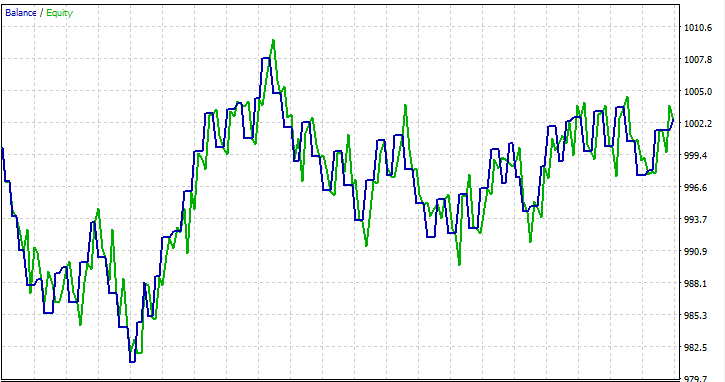
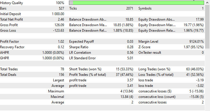
我在一个月 2023.01.01 - 2023.02.01 的开盘价上进行了测试,看看一切是否正常。
交易决策树常见问题解答:
| 问题 | 回答 |
|---|---|
| 输入数据的常规化对决策树重要吗? | 不,常规化对于决策树来说通常根本不重要。决策树根据特征阈值进行拆分,特征的规模不会影响树结构。不过,检查常规化对模型性能的影响是一种很好的做法。 |
| 决策树如何处理交易数据中的类别变化? | 决策树可以从本质上处理类别变化。它们基于是否满足条件(包括类别变化的条件)执行二元拆分。该树将判定类别特征的最优拆分点。 |
| 决策树可以用于交易中的时间序列预测吗? | 虽然决策树可用于交易中的时间序列预测,但它们也许无法像递归神经网络(RNN)等模型那样有效地捕获复杂的现时形态。像随机森林这样的融合方法可以提供更大的稳健性 |
| 决策树是否存在过拟合? | 决策树,尤其是深层决策树,可能很容易因捕获训练数据中的噪声而过拟合。可以采用修剪和限制树的深度等技术来缓解交易应用程序中的过拟合 |
| 决策树是否适合交易模型中的特征重要性分析? | 是的,决策树提供了一种评估特征重要性的本质方法。对于树顶部决策拆分贡献更大的特征通常更为关键。这种分析可以提供对驱动交易决策的因素的见解。 |
| 决策树对交易数据中的异常值有多敏感? | 决策树对异常值可能很敏感,尤其是当树很深时。异常值可能会导致捕获噪声的特定拆分。可以应用预处理步骤(例如异常值检测和移除)来降低这种敏感性。 |
| 在交易模型中,是否需要针对决策树调整特定的超参数? | 是的,需优化的关键超参数包括
可以使用交叉验证来查找给定数据集的最优超参数值。 |
| 决策树可以成为融合方式的一部分吗? | 是的,决策树可以成为随机森林等融合方法的一部分,该方法将多个树组合在一起,从而提高整体预测性能。融合方法在交易应用中通常稳健且有效。 |
决策树的优点:
可解释性:
- 决策树易于理解和解释。树状结构的图形表示,令决策过程的清晰可视化成为可能。
处理非线性:
- 决策树可以捕获数据中的非线性关系,令其适用于非线性决策边界的问题。
处理混合数据类型:
- 决策树可以获取数值和类别数据,而无需进行大量的预处理。
特征重要性:
- 决策树提供了一种评估特征重要性的本质方法,有助于识别影响目标变量的关键因素。
没有关于数据分布的假设:
- 决策树不对数据分布做出任何假设,令其具有多样性,并适用于各种数据集。
对异常值的稳健性:
- 决策树对异常值相对稳健,因为拆分基于相对比较,不受绝对值的影响。
自动变化选择:
- 树构建过程包括自动变化选择,减少了对手工特征工程的需求。
可以处理缺失值:
- 决策树可以处理特征中的缺失值,而无需插补,因为拆分是根据可用数据进行的。
决策树的缺点:
过拟合:
- 决策树容易过拟合,尤其是当它们很深,并在训练数据中捕获到噪声时。可用修剪等技术解决此问题。
不稳定:
- 数据的微小变化可能会导致树结构的重大变化,从而令决策树在某种程度上不稳定。
偏向主导类别:
- 在具有不平衡类别的数据集中,决策树可能会偏向于占主导地位的类别,从而导致少数类的性能欠佳。
全局最优对比局部最优:
- 决策树侧重于在每个节点上找到局部最优拆分,这也许不一定会导致全局最优解。
有限的表现力:
- 与更复杂的模型(如神经网络)相比,决策树可能难以表达数据中的复杂关系。
不适合连续输出:
- 虽然决策树对于分类任务来说已经足够了,但它们可能不适合于需要连续输出的任务。
对嘈杂数据敏感:
- 决策树对嘈杂的数据可能很敏感,异常值可能会导致捕获噪声,而非有意义的形态的特定拆分。
偏向于主导特征:
- 由于拆分的方式不同,具有更多级别或类别的特征可能看起来更关键,这可能会引入偏向。人们可以通过特征缩放等技术来解决这个问题。
就是这些,感谢阅读。
在我的 GitHub 存储库中跟踪开发,并为决策树算法和更多 AI 模型做出贡献:https://github.com/MegaJoctan/MALE5/tree/master
附件:
| tree.mqh | 主要包含文件。内含我们上面讨论的主要决策树代码。 |
| metrics.mqh | 内含测量 ML 模型性能的函数和代码。 |
| matrix_utils.mqh | 内含矩阵操作的附加函数。 |
| preprocessing.mqh | 预处理原始输入数据的函数库,令其适合机器学习模型的使用。 |
| DecisionTree Test.mq5(EA) | 主文件。运行决策树的智能系统。 |
本文由MetaQuotes Ltd译自英文
原文地址: https://www.mql5.com/en/articles/13862
 新手在交易中的10个基本错误