
LSTMニューラルネットワークを用いた時系列予測の作成:価格の正規化と時間のトークン化
はじめに
取引戦略の開発におけるニューラルネットワークの使用を探求したかったので、まずYoutubeのビデオをいくつか見て、このトピックを掘り下げてみました。Pythonでのプログラミングの仕方、例えば文字列の使い方、配列の使い方、OOPの使い方、その他すべての基本的なことから始まるので、比較的分かりにくいものが多かったです。その教育者がコースの核心であるニューラルネットワークと機械学習に取りかかる頃には、特定のライブラリや事前に訓練されたモデルの使い方を説明するだけで、それらがどのように機能するのかを実際に説明することはないだろうということに気がつきました。いろいろ探した結果、Andrej Karpathyのビデオにたどり着きました。特に、彼のビデオ「Let's build GPT: from scratch, in code, spelled out」は、シンプルな数学的概念をコードと組み合わせ、数百行のコードで人間のような知性を実現できることを教えてくれました。 このビデオは、私にとってニューラルネットワークの世界を比較的直感的かつ実践的な方法で解き明かし、そのパワーを直接体験する機会を与えてくれました。ChatGPTがどのように機能するのか、Pythonでどのように書くのかなどを理解するために、彼のチャンネルからいくつかの基本的な理解と、100以上のChatGPTクエリの支援を組み合わせ、私は、予測やエキスパートアドバイザー(EA)の構築にニューラルネットワークを使用する方法論を考え出すことができました。この記事では、その道のりを記録するだけでなく、私が学んだこと、そしてLSTMのようなシンプルなニューラルネットワークが市場予測にどのように使用できるかを示したいと思います。
LSTMの概要
インターネットで検索を始めたとき、時系列予測でのLSTMの使用について説明するいくつかの記事を偶然見つけました。特に、Christopher Olah氏によるcolah's blogで、「Understanding LSTM Networks」を見つけました。Olah氏はそのブログで、LSTMの構造と機能を説明し、標準的なRNNと比較し、覗き穴結合(peephole connection)やGated Recurrent Unit (GRU)などのさまざまなLSTMの変種について論じています。Olah氏は最後に、LSTMがRNNのアプリケーションに与える影響の大きさを強調し、Attentionメカニズムのような将来の進歩を指し示しています。
要するに、従来のニューラルネットワークは、メモリがないため、過去の入力からの文脈を必要とするタスクに苦戦していたのです。RNNは情報を持続させるループを持つことでこの問題に対処していますが、それでも長期的な依存関係の難しさに直面しています。例えば、関連する文脈が何単語も後ろにある文の次の単語を予測することは、標準的なRNNでは難しいです。 長・短期記憶(Long Short Term Memory: LSTM)ネットワークは、回帰型ニューラルネットワーク(Recurrent Neural Network: RNN)の一種であり、RNNに欠けている長期的な依存関係をよりうまく扱えるように設計されています。
LSTMは、セル状態と情報の流れを制御する3種類のゲート(入力、忘却、出力)を含む、より複雑なアーキテクチャを使用することでこれを解決します。この設計により、LSTMは情報を長期間記憶することができ、言語モデリング、音声認識、画像キャプションなどのタスクに非常に有効です。私が興味を持ったのは、LSTMがより長い時間情報を記憶する能力を持つため、同じような値動きをした日の過去の値動きを基に、今日の値動きを予測できるかどうかということです。Adrian Tam氏による別の役に立つ記事に出会いました。その記事は「LSTM for Time Series Prediction in PyTorch」という巧妙なタイトルが付けられており、実用的な例を使って数学とプログラミングの側面をわかりやすく説明してくれました。どの通貨ペアでも将来の値動きを予測するために、それらを適用することに挑戦する十分な自信を持てました。
トークン化と正規化プロセス
私は、ニューラルネットワークを訓練するために、ある1日の中の時間をトークン化し、その中の特定の時間枠の価格を正規化する方法を考案しました。次に、訓練したニューラルネットワークを使用して予測をおこない、最後に予測を非正規化して将来の価格の予測を得る方法を見つけました。このアプローチは、冒頭で紹介したChatGPTのビデオにインスパイアされたものです。LLMも同様の戦略で、テキスト文字列を数値やベクトル表現に変換し、言語処理や応答生成のためのニューラルネットワークを訓練します。私の場合、価格については、ニューラルネットワークに入力するデータは、その日の高値または安値に対する相対的なものであることが望ましいです。私が使用した正規化とトークン化の戦略は、以下のスクリプトに示されており、要約すると以下のようになります。
時間のトークン化
-
秒への換算:このスクリプトは、time列(datetime形式)を受け取り、その日の開始からの経過秒数に変換します。この計算には時間、分、秒が含まれます。
-
1日の端数に対する正規化:得られた秒数を1日の総秒数(86400)で割ります。これは、時間を1日の端数で表すtime_tokenを作成します。次は例です。正午は0.5、つまり1日の50%が終わったことになります。
日次ローリング価格正規化
-
日付によるグループ分け:正規化が取引日ごとに独立しておこなわれるように、データは日付の列でグループ化されています。
-
ローリング高値/安値計算:
- 各グループ(day)について、スクリプトはそれぞれ高値と安値の拡大最大値(rolling_high)と拡大最小値(rolling_low)を計算します。つまり、ローリング高値/安値は、一日を通して新しいデータが入ったときだけ増減します。
-
正規化
- 始値、高値、安値、終値は、normalized_price = (price - rolling_low) / (rolling_high - rolling_low)で正規化されます。
- これは、各価格を、その日のこれまでの最高値と最安値に対して0から1の範囲にスケーリングするものです。
- 正規化は日次ベースでおこなわれ、各日の価格関係を確実に把握すると同時に、複数日にわたる価格変動の影響を正規化が受けないようにします。
-
NaNの処理:NaN値は、ローリング高値/安値が確立される前の日の初めに発生する可能性があります。3つの異なるアプローチを考慮しました。1つ目のアプローチは「ドロップ」、2つ目のアプローチは 「フォワードフィル」、そして3つ目のアプローチは「ゼロへの置き換え」でした。多くのテストと「ドロップ」で苦労した後、ゼロに置き換えることにしました。最終的な目標は、このプロセスをONNXデータ処理パイプラインに変換し、コードを複製せずにMQL5で直接使用して予測をおこなうことだからです。ONNXは入力と出力の形状に関しては比較的厳格であることがわかりました。NaNの値を「ドロップ」すると出力ベクトルの形状が変わってしまうため、MQLでONNXを使用するときに予期せぬエラーが発生します。NaNを置換するためにフォワードフィリング法を使おうとしましたが、これはPandas/NumPyの方法であり、私がニューラルネットワークモデルをONNXに変換するために主に使用したライブラリであるtorchには都合よく訳されません。最終的に、NaNを単純にゼロに置き換えることにしました。これが一番うまくいくように思えました。これにより、変数の形状の問題を回避し、データ処理全体のパイプラインを作成し、それをONNXを介してMQLに実装して、MQL内で予測を取得するプロセス全体を合理化することができます。
要約すると、正規化は日次ベースでおこなわれ、各日の価格関係を確実に把握すると同時に、複数日にわたる価格変動の影響を正規化が受けるのを防ぎます。こうすることで、価格が同じようなスケールになり、モデルがより大きな特徴量に偏るのを防ぐことができます。また、1日の中で変化する変動に対応することもできます。
以下のコードは、上記のプロセスを視覚化するのに役立ちます。この記事のzipファイルをダウンロードすると、このコードは「Visualizing the Normalization and Tokenization Process」というフォルダにあります。ファイル名はvisualizing.pyです。
import torch
import torch.nn as nn
import numpy as np
import pandas as pd
from sklearn.preprocessing import MinMaxScaler
import MetaTrader5 as mt5
import matplotlib.pyplot as plt
import joblib

# Connect to MetaTrader 5
if not mt5.initialize():
    print("Initialize failed")
    mt5.shutdown()

# Load market data
symbol = "EURUSD"
timeframe = mt5.TIMEFRAME_M15
rates = mt5.copy_rates_from_pos(symbol, timeframe, 0, 96)  # Note: 96 represents 1 day or 15*96= 1440 minutes of data (there are 1440 minutes in a day)
mt5.shutdown()

# Convert to DataFrame
data = pd.DataFrame(rates)
data['time'] = pd.to_datetime(data['time'], unit='s')
data.set_index('time', inplace=True)

# Tokenize time
data['time_token'] = (data.index.hour * 3600 + data.index.minute * 60 + data.index.second) / 86400

# Normalize prices on a rolling basis resetting at the start of each day
def normalize_daily_rolling(data):
    data['date'] = data.index.date
    data['rolling_high'] = data.groupby('date')['high'].transform(lambda x: x.expanding(min_periods=1).max())
    data['rolling_low'] = data.groupby('date')['low'].transform(lambda x: x.expanding(min_periods=1).min())

    data['norm_open'] = (data['open'] - data['rolling_low']) / (data['rolling_high'] - data['rolling_low'])
    data['norm_high'] = (data['high'] - data['rolling_low']) / (data['rolling_high'] - data['rolling_low'])
    data['norm_low'] = (data['low'] - data['rolling_low']) / (data['rolling_high'] - data['rolling_low'])
    data['norm_close'] = (data['close'] - data['rolling_low']) / (data['rolling_high'] - data['rolling_low'])

    # Replace NaNs with zeros
    data.fillna(0, inplace=True)
    return data

# Visualize the price before normalization
plt.figure(figsize=(15, 10))

plt.subplot(3, 1, 1)
data['close'].plot()
plt.title('Close Prices')
plt.xlabel('Time')
plt.ylabel('Price')

data = normalize_daily_rolling(data)

# Check for NaNs in the data
if data.isnull().values.any():
    print("Data contains NaNs")
    print(data.isnull().sum())

# Drop unnecessary columns
data = data[['time_token', 'norm_open', 'norm_high', 'norm_low', 'norm_close']]

# Visualize the normalized price
plt.subplot(3, 1, 2)
data['norm_close'].plot()
plt.title('Normalized Close Prices')
plt.xlabel('Time')
plt.ylabel('Normalized Price')

# Visualize Time After Tokenization
plt.subplot(3, 1, 3)
data['time_token'].plot()
plt.title('Time Token')
plt.xlabel('Time')
plt.ylabel('Time Token')

plt.tight_layout()
plt.show()
上のコードを実行すれば、私が思いついたアプローチを実際に見ることができます。以下のプロットでは、6/12/2024の価格から、6/13/2024に重なる取引の全日をプロットしています。この日はCPIとFRBの会合の日でもあり、2つの大きなレッドニュースイベントが同じ日に起こるのは比較的珍しいことです。タイムトークンは1日の終わりにリセットされ、1日を通して直線的に増えていくのがわかります。価格もリセットされますが、プロットでは少し見づらいです。新高値が形成されるたびに、正規化された終値の値は1になります。新安値が形成されると、正規化した終値の値は0になります。

訓練および検証ステップの概要
以下のコードは、特にEURUSD通貨ペアに焦点を当てて、価格を予測するためのLSTM (Long Short-Term Memory)モデルを訓練します。ユーザーはEURUSDを他のペアに変更することができます。
データの準備
- データの取得:MetaTrader 5プラットフォームに接続し、EURUSDの過去の価格データ(高値、安値、始値、終値)を15分間隔で取得します。この場合も、1分、5分、15分など、個人のスタイルに合わせて好みの時間枠を選ぶことができます。
- データの前処理:
- データをPandas DataFrameに変換し、インデックスとしてタイムスタンプを設定します。
- 時間を1日のうちの割合として表すtime_token特徴量を作成します。
- 日々の変動を考慮し、連続的な高値/安値のローリングに基づき、各日の価格を正規化します。
- 欠損値(NAN)をゼロで置き換えます。
- ティックボリューム、実ボリューム、スプレッドなどの不要な列を削除します。
- シーケンスの作成:データを60のタイムステップのシーケンスに構造化します。各シーケンスが入力(X)となり、次の終値がターゲット(Y)となります。
- 分割データ:シーケンスを訓練セット(80%)とテストセット(20%)に分けます。
- テンソルへの変換:モデルの互換性のためにデータをPyTorchテンソルに変換します。
モデルの定義と訓練
- LSTMモデルの定義:LSTMモデルのクラスを作成します。
- シーケンスデータを処理するLSTM層
- 最終的な予測をおこなう線形層
- LSTMの内部状態変数
- 訓練の設定
- 平均二乗誤差(MSE)を最小化すべき損失関数として定義します。
- モデルの重みを調整するためにAdamオプティマイザを使用します。
- 再現性のためのランダムシードを設定します。
- モデルの訓練
- 100エポック(訓練データをフルパス)反復します。
- 訓練セットの各シーケンスについて:
- LSTM の隠された状態をリセットします。
- 予測値を得るためにシーケンスをモデルに通します。
- 予測値と真値の間のMSE損失を計算します。
- モデルの重みを更新するためにバックプロパゲーションをおこないます。
- 10エポックごとに損失を表示します。
- モデルの保存:訓練済みモデルのパラメータを保持します。ファイルはlstm_model.pthとして、LSTM_model_training.pyを実行したフォルダと同じフォルダに保存されます。また、MQL5で直接使用するためにモデルをONNX形式に変換します。ONNXファイルはlstm_model.onnxと呼ばれます。注:予測に必要なベクトルの形状は「seq_length, 1, input_size」で、「60, 1, 5」です。これは、15分間データの60個の過去バーが1つのバッチとして必要であり、5つの値 (time_token、norm_open、norm_high、norm_low、norm_close) がすべて0から1の間であることを示します。この記事の後半で、このモデルで使用するデータ処理パイプラインをONNXで作成するために、このパイプラインを使用します。
評価
- 予測の生成
- モデルを評価モードに切り替えます。
- テストセット内のシーケンスを繰り返し、予測を生成します。
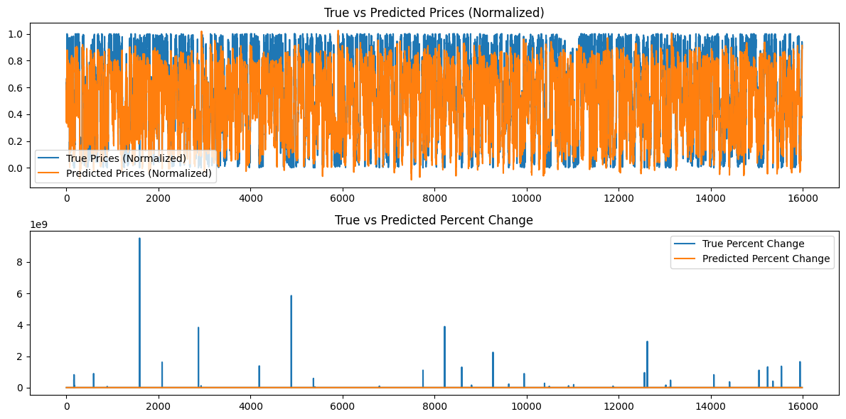
- 結果の視覚化
- 真の正規化価格と予測正規化価格をプロットします。
- 真の値と予測値の両方について、価格の変化率を計算し、プロットします。
モデルパラメータの選択
- このコードの大部分は、日中のトレンドを見つけることに重点を置いて書かれています。しかし、週足、月足など、他の時間枠にも簡単に適応させることができます。私にとって唯一の問題は、データが利用できるかどうかでした。利用できなければ、他の時間枠も含めるようにコードを拡張できたでしょう。
- 15分足を選択したのは、ニューラルネットワークに入力する約80,000本のデータが得られたからです。これは約3年間の取引データ(週末を除く)であり、日中の値動きを予測しようとするまともなLSTMニューラルネットワークを構築するのに十分であると感じました。
- モデルの全体的な基盤は、time_token、norm_open、norm_high、norm_low、norm_closeの5つのパラメータです。したがって、input_size = 5です。私が無視することを選択した追加のパラメータは、ティックボリューム、実ボリューム、スプレッドの3つです。ティックボリュームを除外したのは、信頼できる十分なデータソースが見つからなかったからです。私のブローカーからは実ボリュームを入手できないため、実ボリュームを除外しました。最後に、デモ口座からデータを取得したため、スプレッドはライブ口座のブローカーのスプレッドとは一致しないので除外しました。
- 隠れ層は100を選択しました。これは、うまく機能すると思われる任意の値を選択したものです。
- output_sizeの値が1なのは、このモデルの設計上、次の15分足の予測にしか関心がないからです。
- 私は訓練とテストは80%と20%に分割しました。これも恣意的な選択です。50:50を好む人もいれば、70:30を好む人もいます。自信がなかったので、80:20に分割しました。
- シード値は42を選択しました。私の主な目標は、テストからテストへの結果の再現性を持たせることでした。そのため、シード値を指定したのは、将来的に何らかのパラメータで勝負することになった場合に備えて、結果を均等に比較できるようにするためです。
- 学習率は0.001を選択しました。これもまた恣意的な選択です。ユーザーは自分の学習率を自由に設定できます。
- 配列長(seq_length)は60を選択しました。基本的に、これはLSTMモデルが次のバーについての予測をおこなうために必要な「文脈」のバー数です。これも恣意的な選択でした。60×15分=900分または15時間です。15分足1本を予測できるようになるには、文脈をつかむのに多くの時間が必要で、少し過剰かもしれません。この値を選択する十分な根拠はありませんが、このモデルは柔軟で、ユーザーはこの値を自由に変更することができます。
- 訓練の時間:100エポックを選択したのは、80,000本のバーを使用したモデルを私のコンピュータで実行するには約8時間かかるからです。訓練にはCPUを使用しました。この記事を書きながら、私は何度かコードを改良し、モデルを何度も再実行しなければなりませんでした。モデルに与えられる訓練時間は、8時間が限界でした。
import torch
import torch.nn as nn
import numpy as np
import pandas as pd
import MetaTrader5 as mt5
import matplotlib.pyplot as plt
import torch.onnx
import torch.nn.functional as F

# Connect to MetaTrader 5
if not mt5.initialize():
    print("Initialize failed")
    mt5.shutdown()

# Load market data
symbol = "EURUSD"
timeframe = mt5.TIMEFRAME_M15
rates = mt5.copy_rates_from_pos(symbol, timeframe, 0, 80000)
mt5.shutdown()

# Convert to DataFrame
data = pd.DataFrame(rates)
data['time'] = pd.to_datetime(data['time'], unit='s')
data.set_index('time', inplace=True)

# Tokenize time
data['time_token'] = (data.index.hour * 3600 + data.index.minute * 60 + data.index.second) / 86400

# Normalize prices on a rolling basis resetting at the start of each day
def normalize_daily_rolling(data):
    data['date'] = data.index.date
    data['rolling_high'] = data.groupby('date')['high'].transform(lambda x: x.expanding(min_periods=1).max())
    data['rolling_low'] = data.groupby('date')['low'].transform(lambda x: x.expanding(min_periods=1).min())

    data['norm_open'] = (data['open'] - data['rolling_low']) / (data['rolling_high'] - data['rolling_low'])
    data['norm_high'] = (data['high'] - data['rolling_low']) / (data['rolling_high'] - data['rolling_low'])
    data['norm_low'] = (data['low'] - data['rolling_low']) / (data['rolling_high'] - data['rolling_low'])
    data['norm_close'] = (data['close'] - data['rolling_low']) / (data['rolling_high'] - data['rolling_low'])

    # Replace NaNs with zeros
    data.fillna(0, inplace=True)
    return data

data = normalize_daily_rolling(data)

# Check for NaNs in the data
if data.isnull().values.any():
    print("Data contains NaNs")
    print(data.isnull().sum())

# Drop unnecessary columns
data = data[['time_token', 'norm_open', 'norm_high', 'norm_low', 'norm_close']]

# Create sequences
def create_sequences(data, seq_length):
    xs, ys = [], []
    for i in range(len(data) - seq_length):
        x = data.iloc[i:(i + seq_length)].values
        y = data.iloc[i + seq_length]['norm_close']
        xs.append(x)
        ys.append(y)
    return np.array(xs), np.array(ys)

seq_length = 60
X, y = create_sequences(data, seq_length)

# Split data
split = int(len(X) * 0.8)
X_train, X_test = X[:split], X[split:]
y_train, y_test = y[:split], y[split:]

# Convert to tensors
X_train = torch.tensor(X_train, dtype=torch.float32)
y_train = torch.tensor(y_train, dtype=torch.float32)
X_test = torch.tensor(X_test, dtype=torch.float32)
y_test = torch.tensor(y_test, dtype=torch.float32)

# Set the seed for reproducibility
seed_value = 42
torch.manual_seed(seed_value)

# Define LSTM model class
class LSTMModel(nn.Module):
    def __init__(self, input_size, hidden_layer_size, output_size):
        super(LSTMModel, self).__init__()
        self.hidden_layer_size = hidden_layer_size
        self.lstm = nn.LSTM(input_size, hidden_layer_size)
        self.linear = nn.Linear(hidden_layer_size, output_size)

    def forward(self, input_seq):
        h0 = torch.zeros(1, input_seq.size(1), self.hidden_layer_size).to(input_seq.device)
        c0 = torch.zeros(1, input_seq.size(1), self.hidden_layer_size).to(input_seq.device)
        lstm_out, _ = self.lstm(input_seq, (h0, c0))
        predictions = self.linear(lstm_out.view(input_seq.size(0), -1))
        return predictions[-1]

print(f"Seed value used: {seed_value}")

input_size = 5  # time_token, norm_open, norm_high, norm_low, norm_close
hidden_layer_size = 100
output_size = 1

model = LSTMModel(input_size, hidden_layer_size, output_size)
#model = torch.compile(model)
loss_function = nn.MSELoss()
optimizer = torch.optim.Adam(model.parameters(), lr=0.001)

# Training
epochs = 100
for epoch in range(epochs + 1):
    for seq, labels in zip(X_train, y_train):
        optimizer.zero_grad()
        y_pred = model(seq.unsqueeze(1))

        # Ensure both are tensors of shape [1]
        y_pred = y_pred.view(-1)
        labels = labels.view(-1)

        single_loss = loss_function(y_pred, labels)

        # Print intermediate values to debug NaN loss
        if torch.isnan(single_loss):
            print(f'Epoch {epoch} NaN loss detected')
            print('Sequence:', seq)
            print('Prediction:', y_pred)
            print('Label:', labels)

        single_loss.backward()
        optimizer.step()

    if epoch % 10 == 0 or epoch == epochs:  # Include the final epoch
        print(f'Epoch {epoch} loss: {single_loss.item()}')

# Save the model's state dictionary
torch.save(model.state_dict(), 'lstm_model.pth')

# Convert the model to ONNX format
model.eval()
dummy_input = torch.randn(seq_length, 1, input_size, dtype=torch.float32)
onnx_model_path = "lstm_model.onnx"
torch.onnx.export(model,
                  dummy_input,
                  onnx_model_path,
                  input_names=['input'],
                  output_names=['output'],
                  dynamic_axes={'input': {0: 'sequence'}, 'output': {0: 'sequence'}},
                  opset_version=11)

print(f"Model has been converted to ONNX format and saved to {onnx_model_path}")

# Predictions
model.eval()
predictions = []
for seq in X_test:
    with torch.no_grad():
        predictions.append(model(seq.unsqueeze(1)).item())

# Evaluate the model
plt.plot(y_test.numpy(), label='True Prices (Normalized)')
plt.plot(predictions, label='Predicted Prices (Normalized)')
plt.legend()
plt.show()

# Calculate percent changes with a small value added to the denominator to prevent divide by zero error
true_prices = y_test.numpy()
predicted_prices = np.array(predictions)

true_pct_change = np.diff(true_prices) / (true_prices[:-1] + 1e-10)
predicted_pct_change = np.diff(predicted_prices) / (predicted_prices[:-1] + 1e-10)

# Plot the true and predicted prices
plt.figure(figsize=(12, 6))
plt.subplot(2, 1, 1)
plt.plot(true_prices, label='True Prices (Normalized)')
plt.plot(predicted_prices, label='Predicted Prices (Normalized)')
plt.legend()
plt.title('True vs Predicted Prices (Normalized)')

# Plot the percent change
plt.subplot(2, 1, 2)
plt.plot(true_pct_change, label='True Percent Change')
plt.plot(predicted_pct_change, label='Predicted Percent Change')
plt.legend()
plt.title('True vs Predicted Percent Change')

plt.tight_layout()
plt.show()
モデル評価結果
訓練時間は100エポックで約8時間でした。このモデルはGPUを使用して訓練されたものではありません。自分のPCを使用しました。4年前のゲーミングマシンで、スペックは、AMD Ryzen 5 4600H、Radeon Graphics 3.00GHz、RAM 64GB搭載です。
10エポックごとのシード値と平均二乗誤差損失がコンソールに表示されます。
- 使用したシード値:42
- エポック0の損失:0.01435865368694067
- エポック10の損失:0.014593781903386116
- エポック20の損失:0.02026239037513733
- エポック30の損失:0.017134636640548706
- エポック40の損失:0.017405137419700623
- エポック50の損失:0.004391830414533615
- エポック60の損失:0.0210900716483593
- エポック70の損失:0.008576949127018452
- エポック80の損失:0.019675739109516144
- エポック90の損失:0.008747504092752934
- エポック100の損失:0.033280737698078156
訓練の最後には、以下のような警告も受けました。この警告は、別の方法でモデルを指定することを示唆しています。それを直そうといじくり回しましたが、訓練に時間がかかるため、この警告は無視することにしました。バッチ内のシーケンスの長さは変わらないためです。

さらに、以下のグラフが作成されます。
")
モデル結果の分析
シード値が42の場合のエポックの損失は、不規則に減少しているように見えます。これらは単調ではないので、おそらくモデルはさらなる訓練の恩恵を受けることができるでしょう。あるいは、別のシード値を指定するか、PythonのTorchライブラリによって自動生成されたランダムなシード値を使用し、torch.sEd()コマンドを使用してこの値を出力することも考えられます。さらに、利用可能なデータ量を増やせば、モデルの性能も向上する可能性があります。しかし、そうすることで、ユーザーは、より長い訓練時間やより大きなハードウェアメモリ要件に関連する追加的な計算コストを経験する可能性があります。
生成されたグラフは、15分間のデータ16000本以上を要約しようとするものです。したがって、私が使用したグラフ作成システムでは、ほとんどのデータがつぶれてしまい、評価するのが難しくなるため、あまり効果的ではありません。これらのグラフは、おこなわれた訓練全体をより「グローバル」に表現したものです。そのままでは何の価値もありません。より小さなデータセットでもモデルを訓練し、その役に立ったので、参考のために掲載しましたが、80,000バーの場合、あまり役に立ちません。次のセクションでは、生成されたモデルに基づいて予測をおこなうときにこの問題に対処します。データは「ローカル」表現、つまり日々の価格変動になります。次のセクションでは、60のシーケンス長を利用し、さらに100のバー(15分データの合計160のバー)を追加することによって、モデルに基づいて連続予測を作成し、バー100から0までの連続予測を作成し、おそらくより啓発的なグラフで表現します。
訓練済みモデルを使用して予測をおこなう(Pythonを使用)
予測スクリプトを作成するには、保存されたLSTMモデルを使用して予測をおこなうために、15分足時間枠のEURUSDデータから直近60件の値を使用するのが理想的です。しかし、これを使用する前に素早くモデルを検証できるように、Pythonでグラフとともにローリング予測を得たほうがいいと思いました。以下は、Pythonのユースケースにおける予測スクリプトの主な機能です。スクリプトの概要は以下の通りです。
-
LSTMモデルの定義:スクリプトはLSTMモデルの構造を定義します。このモデルはLSTM層と線形層で構成されています。これは、上記の訓練スクリプトでモデルの訓練に使用したものと同じです。
-
データの準備
- MetaTrader 5に接続し、EURUSDの最新160バー(15分間隔)のデータを取得します。予測に必要な15分足データは60本であるにもかかわらず、160本のバーを引いて予測し、過去100回の予測を比較します。これによって、予測対実績の根本的な傾向がある程度わかるでしょう。
- データはpandas DataFrameに変換され、訓練時に使用されたのと同じローリング正規化手法を用いて正規化されます。
- 時間のトークン化は、時間を数値表現に変換するために適用されます。
-
モデルの読み込み
- 訓練済みLSTMモデル(lstm_model.pthから)が読み込まれます。これは、訓練フェーズで訓練したモデルです。
-
評価
- スクリプトは、データの最後の100ステップを繰り返し実行します。
- 各ステップごとに、60本前のバーを入力とし、モデルを使用して正規化された終値を予測します。
- 真の価格と予測価格は比較のために保存されます。
-
次の予想
- 直近の60本のバーを使用して次のステップの予測をおこないます。
- この予測の変化率を計算します。
- 予想がチャート上に赤い点で表示されます。
-
可視化
- 2つのプロットが作成されます。
- 真 vs. 予測価格(正規化):次の予測がハイライトされています。
- 真 vs. 予測価格パーセント変化:次の予測が強調表示されています。
- Y軸は、より見やすくするために100%を上限としています。
- 2つのプロットが作成されます。
以下のコードはLSTM_model_prediction.pyにあります。このファイルは、この記事に添付されているLSTM_Files.zipのルートにあります。
import torch
import torch.nn as nn
import numpy as np
import pandas as pd
import MetaTrader5 as mt5
import matplotlib.pyplot as plt

# Define LSTM model class (same as during training)
class LSTMModel(nn.Module):
    def __init__(self, input_size, hidden_layer_size, output_size):
        super(LSTMModel, self).__init__()
        self.hidden_layer_size = hidden_layer_size
        self.lstm = nn.LSTM(input_size, hidden_layer_size)
        self.linear = nn.Linear(hidden_layer_size, output_size)
        self.hidden_cell = (torch.zeros(1, 1, self.hidden_layer_size),
                            torch.zeros(1, 1, self.hidden_layer_size))

    def forward(self, input_seq):
        lstm_out, self.hidden_cell = self.lstm(input_seq.view(len(input_seq), 1, -1), self.hidden_cell)
        predictions = self.linear(lstm_out.view(len(input_seq), -1))
        return predictions[-1]

# Normalize prices on a rolling basis resetting at the start of each day
def normalize_daily_rolling(data):
    data['date'] = data.index.date
    data['rolling_high'] = data.groupby('date')['high'].transform(lambda x: x.expanding(min_periods=1).max())
    data['rolling_low'] = data.groupby('date')['low'].transform(lambda x: x.expanding(min_periods=1).min())

    data['norm_open'] = (data['open'] - data['rolling_low']) / (data['rolling_high'] - data['rolling_low'])
    data['norm_high'] = (data['high'] - data['rolling_low']) / (data['rolling_high'] - data['rolling_low'])
    data['norm_low'] = (data['low'] - data['rolling_low']) / (data['rolling_high'] - data['rolling_low'])
    data['norm_close'] = (data['close'] - data['rolling_low']) / (data['rolling_high'] - data['rolling_low'])

    # Replace NaNs with zeros
    data.fillna(0, inplace=True)
    return data[['norm_open', 'norm_high', 'norm_low', 'norm_close']]

# Load the saved model
input_size = 5  # time_token, norm_open, norm_high, norm_low, norm_close
hidden_layer_size = 100
output_size = 1

model = LSTMModel(input_size, hidden_layer_size, output_size)
model.load_state_dict(torch.load('lstm_model.pth'))
model.eval()

# Connect to MetaTrader 5
if not mt5.initialize():
    print("Initialize failed")
    mt5.shutdown()

# Load the latest 160 bars of market data
symbol = "EURUSD"
timeframe = mt5.TIMEFRAME_M15
bars = 160  # 60 for sequence length + 100 for evaluation steps
rates = mt5.copy_rates_from_pos(symbol, timeframe, 0, bars)
mt5.shutdown()

# Convert to DataFrame
data = pd.DataFrame(rates)
data['time'] = pd.to_datetime(data['time'], unit='s')
data.set_index('time', inplace=True)

# Normalize the new data
data[['norm_open', 'norm_high', 'norm_low', 'norm_close']] = normalize_daily_rolling(data)

# Tokenize time
data['time_token'] = (data.index.hour * 3600 + data.index.minute * 60 + data.index.second) / 86400

# Drop unnecessary columns
data = data[['time_token', 'norm_open', 'norm_high', 'norm_low', 'norm_close']]

# Fetch the last 100 sequences for evaluation
seq_length = 60
evaluation_steps = 100

# Initialize lists for storing evaluation results
all_true_prices = []
all_predicted_prices = []

model.eval()

for step in range(evaluation_steps, 0, -1):
    # Get the sequence ending at 'step'
    seq = data.values[-step-seq_length:-step]
    seq = torch.tensor(seq, dtype=torch.float32)

    # Make prediction
    with torch.no_grad():
        model.hidden_cell = (torch.zeros(1, 1, model.hidden_layer_size),
                             torch.zeros(1, 1, model.hidden_layer_size))
        prediction = model(seq).item()

    all_true_prices.append(data['norm_close'].values[-step])
    all_predicted_prices.append(prediction)

# Calculate percent changes and convert to percentages
true_pct_change = (np.diff(all_true_prices) / np.array(all_true_prices[:-1])) * 100
predicted_pct_change = (np.diff(all_predicted_prices) / np.array(all_predicted_prices[:-1])) * 100

# Make next prediction
next_seq = data.values[-seq_length:]
next_seq = torch.tensor(next_seq, dtype=torch.float32)

with torch.no_grad():
    model.hidden_cell = (torch.zeros(1, 1, model.hidden_layer_size),
                         torch.zeros(1, 1, model.hidden_layer_size))
    next_prediction = model(next_seq).item()

# Calculate percent change for the next prediction
next_true_price = data['norm_close'].values[-1]
next_price_pct_change = ((next_prediction - all_predicted_prices[-1]) / all_predicted_prices[-1]) * 100

print(f"Next predicted close price (normalized): {next_prediction}")
print(f"Percent change for the next prediction based on normalized price: {next_price_pct_change:.5f}%")
print("All Predicted Prices: ", all_predicted_prices)

# Plot the evaluation results with capped y-axis
plt.figure(figsize=(12, 8))

plt.subplot(2, 1, 1)
plt.plot(all_true_prices, label='True Prices (Normalized)')
plt.plot(all_predicted_prices, label='Predicted Prices (Normalized)')
plt.scatter(len(all_true_prices), next_prediction, color='red', label='Next Prediction')
plt.legend()
plt.title('True vs Predicted Prices (Normalized, Last 100 Steps)')
plt.ylim(min(min(all_true_prices), min(all_predicted_prices))-0.1, max(max(all_true_prices), max(all_predicted_prices))+0.1)

plt.subplot(2, 1, 2)
plt.plot(true_pct_change, label='True Percent Change')
plt.plot(predicted_pct_change, label='Predicted Percent Change')
plt.scatter(len(true_pct_change), next_price_pct_change, color='red', label='Next Prediction')
plt.legend()
plt.title('True vs Predicted Price Percent Change (Last 100 Steps)')
plt.ylabel('Percent Change (%)')
plt.ylim(-100, 100)  # Cap the y-axis at -100% to 100%

plt.tight_layout()
plt.show()
以下は、コンソールに表示される出力と、得られたグラフです。この予測は、2024年6月14日(ブローカー時間00:45 UTC + 3)の1日の始まりに作成されました。
コンソールの出力:
Next predicted close price (normalized):0.9003118872642517
Percent change for the next prediction based on normalized price:73.64274%
All Predicted Prices: [0.6229779124259949, 0.6659790277481079, 0.6223553419113159, 0.5994003415107727, 0.565409243106842, 0.5767043232917786, 0.5080181360244751, 0.5245669484138489, 0.6399291753768921, 0.5184902548789978, 0.6269711256027222, 0.6532717943191528, 0.7470211386680603, 0.6783792972564697, 0.6942530870437622, 0.6399927139282227, 0.5649009943008423, 0.6392825841903687, 0.6454082727432251, 0.4829435348510742, 0.5231367349624634, 0.17141318321228027, 0.3651347756385803, 0.2568517327308655, 0.41483253240585327, 0.43905267119407654, 0.40459558367729187, 0.25486069917678833, 0.3488359749317169, 0.41225481033325195, 0.13895493745803833, 0.21675345301628113, 0.04991495609283447, 0.28392884135246277, 0.17570143938064575, 0.34913408756256104, 0.17591500282287598, 0.33855849504470825, 0.43142321705818176, 0.5618296265602112, 0.0774659514427185, 0.13539350032806396, 0.4843936562538147, 0.5048894882202148, 0.8364744186401367, 0.782444417476654, 0.7968958616256714, 0.7907949686050415, 0.5655181407928467, 0.6196668744087219, 0.7133172750473022, 0.5095566511154175, 0.3565239906311035, 0.2686333656311035, 0.3386841118335724, 0.5644893646240234, 0.23622554540634155, 0.3433009088039398, 0.3493557274341583, 0.2939424216747284, 0.08992069959640503, 0.33946871757507324, 0.20876094698905945, 0.4227801263332367, 0.4044940173625946, 0.654332160949707, 0.49300187826156616, 0.6266812086105347, 0.807404637336731, 0.5183461904525757, 0.46170246601104736, 0.24424996972084045, 0.3224128782749176, 0.5156376957893372, 0.06813174486160278, 0.1865384578704834, 0.15443122386932373, 0.300825834274292, 0.28375834226608276, 0.4036571979522705, 0.015333771705627441, 0.09899216890335083, 0.16346102952957153, 0.27330827713012695, 0.2869266867637634, 0.21237093210220337, 0.35913240909576416, 0.4736405313014984, 0.3459511995315552, 0.47014304995536804, 0.3305799663066864, 0.47306257486343384, 0.4134630858898163, 0.4199170768260956, 0.5666837692260742, 0.46681761741638184, 0.35662856698036194, 0.3547590374946594, 0.5447400808334351, 0.5184851884841919]

予測結果の分析
コンソールの出力は0.9003118872642517で、これは次の値動きが現在の日足レンジの0.9、つまりおよそ1.07402と1.07336の間、または~8ピップになる可能性が高いことを示しています。これは価格変更としては十分ではないかもしれません。この記事を書いている時点では、2024年6月14日の取引はまだ45分しかおこなわれていなかったため、これは分かります。しかし、このモデルは価格が現在の日足レンジの上限付近で引けると予測しています。
次の行: Percent change for the next prediction based on normalized price:73.64274% - これは、次の価格変動が前の価格より約+74%高くなる可能性があることを示唆しています。1日の値幅が8pipsだとすると、取引をおこなうのに十分なpips数を提供できない可能性があります。
数字や分数を扱う代わりに、ユーザーは、日足(高値-安値)を取り、それに正規化された終値予測値を掛けて、予想できる実際のpipsの値を得る線を追加することを考えるかもしれません。スクリプトをMQLに変換する際、これをおこなうだけでなく、正確な価格予測も得ることができます。
上の出力でわかるように、100の予測リストもコンソールに出力されます。特にMQL5に移行し、そこでスクリプトを使い始めるときには、これらの値を検証に使用することができます。
最後に、PythonのMatplotlibライブラリからグラフを取得し、過去100回の予測をグラフ化し、正規化された基準(0から1のスケール)で終値の実際の変化と比較します。赤い点は、正規化された基準で次に最も可能性の高い価格を示しており、次に起こり得る価格の方向の目安を示しています。この特定の日のデータに基づくと、私たちの予測は市場に遅れをとっているようで、予測結果がその日の実際の値動きとうまく一致していない可能性があることを示しています。このような日には、裁量トレーダーやユーザーは、モデルが正確な予測をおこなわないため、取引をおこなわず、傍観することを検討すべきです。これは必ずしもデータセット全体にわたってモデルの予測が正しくないことを意味しないので、再訓練は必要ないかもしれません。
PythonからONNXへの移行とMQL5での訓練済みモデルの直接使用
データ処理パイプラインの作成
データ処理パイプラインを作る際に考えたのは、Pythonで作成した正規化とトークン化のコードを複製しないことでした。MQLでそのコードを書き直したくありませんでした。そこで、スクリプトをデータパイプラインに変換し、ONNXに変換して、ONNXを直接MQLのデータ処理に使用することにしました。データ処理パイプラインを作成した経験がないため、このコードを理解するのに数日かかりました。私が苦労した理由は、Pythonはデータ型に関して比較的柔軟だということです。しかし、ONNXに変換する場合は、より厳格で具体的でなければなりません。途中で何度もエラーに遭遇しました。最終的に、それを理解したとき、私はとても嬉しかったので、以下のスクリプトを共有できることを嬉しく思います。このスクリプトがどのように機能するのか、簡単にまとめてみました。
先に述べたように、前処理は2つの重要なステップからなります。
-
時間のトークン化:生の時刻(例えば午後3時45分)を0から1の間の分数値に変換し、24時間経過した1日の部分を表します。
-
日次ローリング正規化:このプロセスは、価格データ(始値、高値、安値、終値)を日次ベースで標準化します。各日における最低価格と最高価格を計算し、これらの値を基準に価格を正規化します。この正規化は、価格データが一貫したスケールを持っていることを保証することで、モデルの訓練に役立ちます。
コンポーネント
-
TimeTokenizer(カスタムTransformer):このクラスは時間のトークン化を処理します。これは入力テンソルから時間列を抽出し、それを一日の分数表現に変換し、他の価格データと結合します。
-
DailyRollingNormalizer(カスタムTransformer):このクラスは、毎日のローリング正規化をおこないます。価格データを繰り返し、各日の最大値と最小値を記録します。その後、これらの動的な値を使用して価格が正規化されます。また、計算中に発生する可能性のあるNaN値を置き換えるステップも含まれています。
-
ReplaceNaNs (カスタムTransformer):計算で得られたすべての NaN 値をゼロに置き換えます。
-
パイプライン(nn.Sequential):これは、上記の3つのカスタムTransformerをシーケンシャルなワークフローに組み合わせたものです。入力データは、TimeTokenizer、DailyRollingNormalizer、ReplaceNaNsの順に通過します。
-
MetaTrader5 Connection:このスクリプトは、EUR/USD の過去の価格データを取得するために MetaTrader 5 への接続を確立します。
実行
-
データの読み込み:このスクリプトは、MetaTrader 5からEURUSDペアの15分足で160本のバー(価格データポイント)を取得します。
-
データ変換:生データは、さらなる処理のためにPyTorchテンソルに変換されます。
-
パイプライン処理:このテンソルは、定義されたパイプラインを通過し、時間トークン化と日次ローリング正規化のステップが適用されます。
-
ONNXエクスポート:最終的に前処理されたデータはコンソールに出力され、処理前と処理後の結果が表示されます。さらに、前処理パイプライン全体がONNXファイルにエクスポートされます。ONNXは、機械学習モデルを異なる枠組みや環境間で簡単に転送できるオープンな形式であり、モデルの展開と使用における幅広い互換性を保証します。
重要なポイント
- モジュール性:カスタムTransformerを使用することで、コードがモジュール化され、再利用可能になります。各Transformerは、特定の前処理ステップをカプセル化します。
- PyTorch:このスクリプトは、テンソル演算とモデル管理のために、一般的な深層学習枠組みであるPyTorchに依存しています。
- ONNXエクスポート:ONNXにエクスポートすることで、前処理ステップを、訓練済みモデルが配置される異なるプラットフォームやツールにシームレスに統合できます。
import torch
import torch.nn as nn
import pandas as pd
import MetaTrader5 as mt5

# Custom Transformer for tokenizing time
class TimeTokenizer(nn.Module):
    def forward(self, X):
        time_column = X[:, 0]  # Assuming 'time' is the first column
        time_token = (time_column % 86400) / 86400
        time_token = time_token.unsqueeze(1)  # Add a dimension to match the input shape
        return torch.cat((time_token, X[:, 1:]), dim=1)  # Concatenate the time token with the rest of the input

# Custom Transformer for daily rolling normalization
class DailyRollingNormalizer(nn.Module):
    def forward(self, X):
        time_tokens = X[:, 0]  # Assuming 'time_token' is the first column
        price_columns = X[:, 1:]  # Assuming 'open', 'high', 'low', 'close' are the remaining columns

        normalized_price_columns = torch.zeros_like(price_columns)
        rolling_max = price_columns.clone()
        rolling_min = price_columns.clone()

        for i in range(1, price_columns.shape[0]):
            reset_mask = (time_tokens[i] < time_tokens[i-1]).float()
            rolling_max[i] = reset_mask * price_columns[i] + (1 - reset_mask) * torch.maximum(rolling_max[i-1], price_columns[i])
            rolling_min[i] = reset_mask * price_columns[i] + (1 - reset_mask) * torch.minimum(rolling_min[i-1], price_columns[i])
            denominator = rolling_max[i] - rolling_min[i]
            normalized_price_columns[i] = (price_columns[i] - rolling_min[i]) / denominator

        time_tokens = time_tokens.unsqueeze(1)  # Assuming 'time_token' is the first column
        return torch.cat((time_tokens, normalized_price_columns), dim=1)

class ReplaceNaNs(nn.Module):
    def forward(self, X):
        X[torch.isnan(X)] = 0
        X[X != X] = 0  # replace negative NaNs with 0
        return X

# Connect to MetaTrader 5
if not mt5.initialize():
    print("Initialize failed")
    mt5.shutdown()

# Load market data (reduced sample size for demonstration)
symbol = "EURUSD"
timeframe = mt5.TIMEFRAME_M15
rates = mt5.copy_rates_from_pos(symbol, timeframe, 0, 160) #intialize with maximum number of bars allowed by your broker
mt5.shutdown()

# Convert to DataFrame and keep only 'time', 'open', 'high', 'low', 'close' columns
data = pd.DataFrame(rates)[['time', 'open', 'high', 'low', 'close']]

# Convert the DataFrame to a PyTorch tensor
data_tensor = torch.tensor(data.values, dtype=torch.float32)

# Create the updated pipeline
pipeline = nn.Sequential(
    TimeTokenizer(),
    DailyRollingNormalizer(),
    ReplaceNaNs()
)

# Print the data before processing
print('Data Before Processing\n', data[:100])

# Process the data
processed_data = pipeline(data_tensor)

print('Data After Processing\n', processed_data[:100])

# Export the pipeline to ONNX format
dummy_input = torch.randn(len(data), len(data.columns))
torch.onnx.export(pipeline, dummy_input, "data_processing_pipeline.onnx", input_names=["input"], output_names=["output"])
コードからの出力は、処理前と処理後のデータがコンソールに表示されます。その出力は重要ではないのでここでは再現しません。出力を見るためにはご自分でスクリプトを実行してください。さらに、出力はdata_processing_pipeline.onnxというファイルを作成します。このONNXモデルで使用されている形状を検証するために、次のようなスクリプトを作成しました。
このスクリプトは「ONNX Data Pipeline」フォルダにあり、shape_check.pyと呼ばれています。これらのファイルは、この記事に添付されているLSTM_Files.zipにあります。
import onnx

model = onnx.load("data_processing_pipeline.onnx")
onnx.checker.check_model(model)

for input in model.graph.input:
    print(f'Input name: {input.name}')
    print(f'Input type: {input.type}')
    for dim in input.type.tensor_type.shape.dim:
        print(dim.dim_value)
結果は次のようになります。
- 160
- 5
したがって、このモデルで必要とされる形状は、160-15分バー、5つの値(UNIX整数としての時間値、始値、高値、安値、終値)です。データ処理の結果、正規化されたデータはtime_token、norm_open、norm_high、norm_low、norm_closeとなります。
MQLでのデータ処理をテストするために、データが当初意図したとおりに変換されていることを検証するための特定のスクリプトも作成しました。添付のzipファイルのルートフォルダにある「LSTM Data Pipeline.mq5」です。このスクリプトは以下にあります。主な特徴は以下の通りです。
-
初期化(OnInit)
- リソースとして埋め込まれたバイナリデータ(data_processing_pipeline.onnx)からONNXモデルを読み込みます。注:ONNXモデルはLSTMというフォルダの中に格納されており、下図のようにExpertsフォルダのサブフォルダになっています。
- 次に、ONNXコードに基づいてモデルの入力と出力の形状を設定します。そのため、「LSTM Data Pipeline Test.ex5」はExpertsフォルダに格納する必要があります。他の方法でファイルを保存する場合は、この行を更新してコードが適切に動作するようにしてください。
-
#resource "\\LSTM\\data_processing_pipeline.onnx" as uchar ExtModel[]

-
ティックデータ処理(OnTick)
- この関数は価格ティックの更新ごとにトリガーされます。
- 次のバー(この場合は15分足のローソク足)が形成されるまで待ちます。
- ProcessData関数を呼び出し、データの処理と予測をおこないます。
-
データ処理(ProcessData)
- EURUSD M15データの最新の SAMPLE_SIZE(ここでは 160)バーを取得します。
- 取得したデータから、時間、始値、高値、安値、終値を抽出します。
- 時間成分を正規化し、1日の端数を表します(0から1の間)。
- ONNXモデルの入力データを1次元ベクトルとして準備します。
- 用意された入力ベクトルでONNXモデル(OnnxRun)を実行します。
- モデルから処理された出力を受け取ります。
- 時間トークンと正規化された価格を含む、処理されたデータを出力します。
//+------------------------------------------------------------------+
//|                                                  ONNX Test       |
//|                                                   Copyright 2023 |
//|                                               Your Name Here     |
//+------------------------------------------------------------------+
#property copyright   "Copyright 2023, Your Name Here"
#property link        "https://www.mql5.com"
#property version     "1.00"

static vectorf ExtOutputData(1);
vectorf output_data(1);

#include <Trade\Trade.mqh>
CTrade trade;

#resource "\\LSTM\\data_processing_pipeline.onnx" as uchar ExtModel[]

#define SAMPLE_SIZE 160  // Adjusted to match the model's expected input size

long     ExtHandle=INVALID_HANDLE;
datetime ExtNextBar=0;

// Expert Advisor initialization
int OnInit()
{
   // Load the ONNX model
   ExtHandle = OnnxCreateFromBuffer(ExtModel, ONNX_DEFAULT);
   if (ExtHandle == INVALID_HANDLE)
   {
      Print("Error creating model OnnxCreateFromBuffer ", GetLastError());
      return(INIT_FAILED);
   }

   // Set input shape


   const long input_shape[] = {SAMPLE_SIZE, 5};  // Adjust based on your model's input dimensions
   if (!OnnxSetInputShape(ExtHandle, ONNX_DEFAULT, input_shape))
   {
      Print("Error setting the input shape OnnxSetInputShape ", GetLastError());
      return(INIT_FAILED);
   }

   // Set output shape
   const long output_shape[] = {SAMPLE_SIZE, 5};  // Adjust based on your model's output dimensions
   if (!OnnxSetOutputShape(ExtHandle, 0, output_shape))
   {
      Print("Error setting the output shape OnnxSetOutputShape ", GetLastError());
      return(INIT_FAILED);
   }

   return(INIT_SUCCEEDED);
}

// Expert Advisor deinitialization
void OnDeinit(const int reason)
{
   if (ExtHandle != INVALID_HANDLE)
   {
      OnnxRelease(ExtHandle);
      ExtHandle = INVALID_HANDLE;
   }
}

// Process the tick function
void OnTick()
{
   if (TimeCurrent() < ExtNextBar)
      return;

   ExtNextBar = TimeCurrent();
   ExtNextBar -= ExtNextBar % PeriodSeconds();
   ExtNextBar += PeriodSeconds();

   // Fetch new data and run the ONNX model
   if (!ProcessData())
   {
      Print("Error processing data");
      return;
   }
}

// Function to process data using the ONNX model
bool ProcessData()
{
   MqlRates rates[SAMPLE_SIZE];
   int copied = CopyRates(_Symbol, PERIOD_M15, 1, SAMPLE_SIZE, rates);
   if (copied != SAMPLE_SIZE)
   {
      Print("Failed to copy the expected number of rates. Expected: ", SAMPLE_SIZE, ", Copied: ", copied);
      return false;
   }
   else if(copied == SAMPLE_SIZE)
   {
      Print("Successfully copied the expected number of rates. Expected: ", SAMPLE_SIZE, ", Copied: ", copied);
   }

   double min_time = rates[0].time;
   double max_time = rates[0].time;
   for (int i = 1; i < copied; i++)
   {
      if (rates[i].time < min_time)
         min_time = rates[i].time;
      if (rates[i].time > max_time)
         max_time = rates[i].time;
   }

   float input_data[SAMPLE_SIZE * 5];
   int count;
   for (int i = 0; i < copied; i++)
   {
      count++;
      // Normalize time to be between 0 and 1 within a day
      input_data[i * 5 + 0] = (float)((rates[i].time));  // normalized time
      input_data[i * 5 + 1] = (float)rates[i].open;  // open
      input_data[i * 5 + 2] = (float)rates[i].high;  // high
      input_data[i * 5 + 3] = (float)rates[i].low;   // low
      input_data[i * 5 + 4] = (float)rates[i].close; // close
   }
   Print("Count of copied after for loop: ", count);
   // Resize input vector to match the copied data size
   vectorf input_vector;
   input_vector.Resize(copied * 5);
   for (int i = 0; i < copied * 5; i++)
   {
      input_vector[i] = input_data[i];
   }

   vectorf output_vector;
   output_vector.Resize(copied * 5);

   if (!OnnxRun(ExtHandle, ONNX_NO_CONVERSION, input_vector, output_vector))
   {
      Print("Error running the ONNX model: ", GetLastError());
      return false;
   }

   // Process the output data as needed
   for (int i = 0; i < copied; i++)
   {
      float time_token = output_vector[i * 5 + 0];
      float norm_open = output_vector[i * 5 + 1];
      float norm_high = output_vector[i * 5 + 2];
      float norm_low = output_vector[i * 5 + 3];
      float norm_close = output_vector[i * 5 + 4];

      // Print the processed data
      PrintFormat("Time Token: %f, Norm Open: %f, Norm High: %f, Norm Low: %f, Norm Close: %f",
                  time_token, norm_open, norm_high, norm_low, norm_close);
   }

   return true;
}
このスクリプトの出力は以下の通りです。データパイプラインが期待通りに機能していることを検証します。

上記の出力を再確認するために、Pythonで「LSTM Data Pipeline Test.py」という追加のスクリプトを作成しました。このスクリプトは、この記事の最後に添付したzipファイル(「ONNX Data Pipeline」フォルダ)にも含まれており、簡単に確認できるように以下に記載されています。
import torch
import onnx
import onnxruntime as ort
import MetaTrader5 as mt5
import pandas as pd
import numpy as np

# Load the ONNX model
onnx_model = onnx.load("data_processing_pipeline.onnx")
onnx.checker.check_model(onnx_model)

# Initialize MT5 and fetch new data
if not mt5.initialize():
    print("Initialize failed")
    mt5.shutdown()

symbol = "EURUSD"
timeframe = mt5.TIMEFRAME_M15
rates = mt5.copy_rates_from_pos(symbol, timeframe, 0, 160)
mt5.shutdown()

# Convert the new data to a DataFrame
data = pd.DataFrame(rates)[['time', 'open', 'high', 'low', 'close']]
data_tensor = torch.tensor(data.values, dtype=torch.float32)

# Prepare the input for ONNX
input_data = data_tensor.numpy()

# Run the ONNX model
ort_session = ort.InferenceSession("data_processing_pipeline.onnx")
input_name = ort_session.get_inputs()[0].name
output_name = ort_session.get_outputs()[0].name

processed_data = ort_session.run([output_name], {input_name: input_data})[0]

# Convert the output back to DataFrame for easy viewing
processed_df = pd.DataFrame(processed_data, columns=['time_token', 'norm_open', 'norm_high', 'norm_low', 'norm_close'])

print('Processed Data')
print(processed_df)
上記のスクリプトを実行したときの出力を以下に示します。出力形式と形状は、上記のMQL出力で見たものと同じです。

MQLにおける予測のための訓練済みモデルの使用
このセクションでは、最終的に、この記事の異なる部分であるデータ処理と予測を1つのスクリプトにつなげ、ユーザーがモデルを訓練した後に予測を得られるようにしたいと思います。MQLで予想を立て、EAを作成するために必要なことを簡単におさらいしましょう。
- LSTM_model_training.pyを実行してモデルを訓練します。パラメータは自由に調整できます。このファイルを実行すると、lstm_model.onnxが作成されます。
- LSTM_model_training.pyを実行して出力されたlstm_model.onnxファイルをMQL ExpertsフォルダのLSTMサブフォルダにコピーします。
- LSTM Data Pipeline.pyを実行してデータ処理パイプラインを作成します。このファイルは、添付のZIPファイル内の「ONNX Data Pipeline」フォルダ内にあります。
- このファイルを実行すると、データ処理用のONNXファイルが作成されます。data_processing_pipeline.onnxをMQL ExpertsフォルダのLSTMサブフォルダにコピーします。
- 以下のスクリプトをメインのExpertsフォルダに保存し、EURUSD 15分足チャートに添付して予測を得ます。
//+------------------------------------------------------------------+
//|                                                  ONNX Test       |
//|                                                   Copyright 2023 |
//|                                               Your Name Here     |
//+------------------------------------------------------------------+
#property copyright   "Copyright 2023, Your Name Here"
#property link        "https://www.mql5.com"
#property version     "1.00"

static vectorf ExtOutputData(1);
vectorf output_data(1);

#include <Trade\Trade.mqh>
//#include <Chart\Chart.mqh>
CTrade trade;

#resource "\\LSTM\\data_processing_pipeline.onnx" as uchar DataProcessingModel[]
#resource "\\LSTM\\lstm_model.onnx" as uchar PredictionModel[]

#define SAMPLE_SIZE_DATA 160  // Adjusted to match the model's expected input size
#define SAMPLE_SIZE_PRED 60

long     DataProcessingHandle = INVALID_HANDLE;
long     PredictionHandle = INVALID_HANDLE;
datetime ExtNextBar = 0;

// Expert Advisor initialization
int OnInit()
{
   // Load the data processing ONNX model
   DataProcessingHandle = OnnxCreateFromBuffer(DataProcessingModel, ONNX_DEFAULT);
   if (DataProcessingHandle == INVALID_HANDLE)
   {
      Print("Error creating data processing model OnnxCreateFromBuffer ", GetLastError());
      return(INIT_FAILED);
   }

   // Set input shape for data processing model
   const long input_shape[] = {SAMPLE_SIZE_DATA, 5};  // Adjust based on your model's input dimensions
   if (!OnnxSetInputShape(DataProcessingHandle, ONNX_DEFAULT, input_shape))
   {
      Print("Error setting the input shape OnnxSetInputShape for data processing model ", GetLastError());
      return(INIT_FAILED);
   }

   // Set output shape for data processing model
   const long output_shape[] = {SAMPLE_SIZE_DATA, 5};  // Adjust based on your model's output dimensions
   if (!OnnxSetOutputShape(DataProcessingHandle, 0, output_shape))
   {
      Print("Error setting the output shape OnnxSetOutputShape for data processing model ", GetLastError());
      return(INIT_FAILED);
   }

   // Load the prediction ONNX model
   PredictionHandle = OnnxCreateFromBuffer(PredictionModel, ONNX_DEFAULT);
   if (PredictionHandle == INVALID_HANDLE)
   {
      Print("Error creating prediction model OnnxCreateFromBuffer ", GetLastError());
      return(INIT_FAILED);
   }

   // Set input shape for prediction model
   const long prediction_input_shape[] = {SAMPLE_SIZE_PRED, 1, 5};  // Adjust based on your model's input dimensions
   if (!OnnxSetInputShape(PredictionHandle, ONNX_DEFAULT, prediction_input_shape))
   {
      Print("Error setting the input shape OnnxSetInputShape for prediction model ", GetLastError());
      return(INIT_FAILED);
   }

   // Set output shape for prediction model
   const long prediction_output_shape[] = {1};  // Adjust based on your model's output dimensions
   if (!OnnxSetOutputShape(PredictionHandle, 0, prediction_output_shape))
   {
      Print("Error setting the output shape OnnxSetOutputShape for prediction model ", GetLastError());
      return(INIT_FAILED);
   }

   return(INIT_SUCCEEDED);
}

// Expert Advisor deinitialization
void OnDeinit(const int reason)
{
   if (DataProcessingHandle != INVALID_HANDLE)
   {
      OnnxRelease(DataProcessingHandle);
      DataProcessingHandle = INVALID_HANDLE;
   }

   if (PredictionHandle != INVALID_HANDLE)
   {
      OnnxRelease(PredictionHandle);
      PredictionHandle = INVALID_HANDLE;
   }
}

// Process the tick function
void OnTick()
{
   if (TimeCurrent() < ExtNextBar)
      return;

   ExtNextBar = TimeCurrent();
   ExtNextBar -= ExtNextBar % PeriodSeconds();
   ExtNextBar += PeriodSeconds();

   // Fetch new data and run the data processing ONNX model
   vectorf input_data = ProcessData(DataProcessingHandle);
   if (input_data.Size() == 0)
   {
      Print("Error processing data");
      return;
   }

   // Make predictions using the prediction ONNX model
   double predictions[SAMPLE_SIZE_DATA - SAMPLE_SIZE_PRED + 1];
   for (int i = 0; i < SAMPLE_SIZE_DATA - SAMPLE_SIZE_PRED + 1; i++)
   {
      double prediction = MakePrediction(input_data, PredictionHandle, i, SAMPLE_SIZE_PRED);
      //if (prediction < 0)
      //{
      //   Print("Error making prediction");
      //   return;
      //}

      // Print the prediction
      //PrintFormat("Predicted close price (index %d): %f", i, prediction);
      double min_price = iLow(Symbol(), PERIOD_D1, 0); //price is relative to the day's price therefore we use low of day for min price
      double max_price = iHigh(Symbol(), PERIOD_D1, 0); //high of day for max price
      double price = prediction * (max_price - min_price) + min_price;
      predictions[i] = price;
      PrintFormat("Predicted close price (index %d): %f", i, predictions[i]);
   }

   // Get the actual prices for the last 60 bars
   double actual_prices[SAMPLE_SIZE_PRED];
   for (int i = 0; i < SAMPLE_SIZE_PRED; i++)
   {
      actual_prices[i] = iClose(Symbol(), PERIOD_M15, SAMPLE_SIZE_PRED - i);
      Print(actual_prices[i]);
   }

   // Create a label object to display the predicted and actual prices
   string label_text = "Predicted | Actual\n";
   for (int i = 0; i < SAMPLE_SIZE_PRED; i++)
   {
      label_text += StringFormat("%.5f | %.5f\n", predictions[i], actual_prices[i]);
   }

   label_text += StringFormat("Next prediction: %.5f", predictions[SAMPLE_SIZE_DATA - SAMPLE_SIZE_PRED]);
   Print(label_text);
   //int label_handle = ObjectCreate(OBJ_LABEL, 0, 0, 0);
   //ObjectSetText(label_handle, label_text, 12, clrWhite, clrBlack, ALIGN_LEFT);
   //ObjectMove(label_handle, 0, ChartHeight() - 20, ChartWidth(), 20);

}

// Function to process data using the data processing ONNX model
vectorf ProcessData(long data_processing_handle)
{
   MqlRates rates[SAMPLE_SIZE_DATA];
   vectorf blank_vector;
   int copied = CopyRates(_Symbol, PERIOD_M15, 1, SAMPLE_SIZE_DATA, rates);
   if (copied != SAMPLE_SIZE_DATA)
   {
      Print("Failed to copy the expected number of rates. Expected: ", SAMPLE_SIZE_DATA, ", Copied: ", copied);
      return blank_vector;
   }

   float input_data[SAMPLE_SIZE_DATA * 5];
   for (int i = 0; i < copied; i++)
   {
      // Normalize time to be between 0 and 1 within a day
      input_data[i * 5 + 0] = (float)((rates[i].time));  // normalized time
      input_data[i * 5 + 1] = (float)rates[i].open;  // open
      input_data[i * 5 + 2] = (float)rates[i].high;  // high
      input_data[i * 5 + 3] = (float)rates[i].low;   // low
      input_data[i * 5 + 4] = (float)rates[i].close; // close
   }

   vectorf input_vector;
   input_vector.Resize(copied * 5);
   for (int i = 0; i < copied * 5; i++)
   {
      input_vector[i] = input_data[i];
   }

   vectorf output_vector;
   output_vector.Resize(copied * 5);

   if (!OnnxRun(data_processing_handle, ONNX_NO_CONVERSION, input_vector, output_vector))
   {
      Print("Error running the data processing ONNX model: ", GetLastError());
      return blank_vector;
   }

   return output_vector;
}

// Function to make predictions using the prediction ONNX model
double MakePrediction(const vectorf& input_data, long prediction_handle, int start_index, int size)
{
   vectorf input_subset;
   input_subset.Resize(size * 5);
   for (int i = 0; i < size * 5; i++)
   {
      input_subset[i] = input_data[start_index * 5 + i];
   }

   vectorf output_vector;
   output_vector.Resize(1);

   if (!OnnxRun(prediction_handle, ONNX_NO_CONVERSION, input_subset, output_vector))
   {
      Print("Error running the prediction ONNX model: ", GetLastError());
      return -1.0;
   }

   // Extract the normalized close price from the output data
   double norm_close = output_vector[0];

   return norm_close;
}
この記事で説明したのとは異なるフォルダ構造を使用している場合は、以下のコード行を自分のフォルダやファイルのパスに合うように変更してください。
#resource "\\LSTM\\data_processing_pipeline.onnx" as uchar DataProcessingModel[]
#resource "\\LSTM\\lstm_model.onnx" as uchar PredictionModel[]
おさらいしておくと、スクリプトの仕組みはこうです。15分足のEURUSDで動作します。
-
データ前処理モデル:このモデル(data_processing_pipeline.onnx)は、時間のトークン化(時間を数値表現に変換する)や価格データの正規化などのタスクを処理し、訓練済みLSTMモデルで使用できるように準備します。
-
予測モデル:このモデル(lstm_model.onnx)はLSTMモデル(Long Short-Term Memory)ネットワークで、15分足で過去60本の値動きを分析し、次の終値の可能性を予測します。
機能性
-
初期化(OnInit)
- 組み込みリソースからONNXモデル(データ前処理と予測)の両方を読み込みます。
- 両モデルの入出力形状を、それぞれの要件に基づいて設定します。
-
ティックデータ処理(OnTick)
- この関数は、新しい価格ティックごとにトリガーされます。
- 次の15分足バー(ローソク足)が形成されるまで待ちます。
- ProcessData関数を呼び出し、データの前処理をおこないます。
- MakePrediction関数を使用して価格予測を生成し、前処理されたデータを繰り返し処理します。
- 正規化された予測値を実際の価格値に戻します。注:予測用のMQLでは、現在以下のコード行を使用しています。これらのコード行は、日々の高値と安値を0から1の間で正規化した予測値を、実際の目標価格に変換します。
-
double min_price = iLow(Symbol(), PERIOD_D1, 0); //price is relative to the day's price therefore we use low of day for min price
double max_price = iHigh(Symbol(), PERIOD_D1, 0); //high of day for max price
double price = prediction * (max_price - min_price) + min_price;
- 予測終値と実際の終値を比較するために表示します。数値は[操作ログ]タブで確認できます。
- 予測価格と実際の価格の情報を文字列で書式設定します。
- 注:コメントされたコード部分は、予測値と実際の値を表示するためにチャートにラベルを作成するように設計されているようです。これは、リアルタイムでモデルのパフォーマンスを評価するための視覚的な補助となるでしょう。しかし、まだコードを完成させることができませんでした。というのも、指標として、あるいはEAとして、予測をどのように使用するのがベストなのか、まだ考えているからです。
-
データ処理(ProcessData)
- EURUSDのM15データの最新160バーを取得します。
- データ処理モデルの入力データを準備します(時間、始値、高値、安値、終値)。
- データ処理モデルを実行し、入力データの正規化とトークン化をおこないます。
-
予測(MakePrediction)
- 前処理済みデータのサブセット(60点のデータ列)を入力とします。
- 予測モデルを実行し、正規化された予測終値を連続的に取得します。
- 予想を出力します([エキスパート]タブで確認できます)。
以下が出力形式です。

見ての通り、出力としていくつかの異なるものが得られます。まず、[Next Prediction]の上の列に予測値と実際の値が表示されます。上記のコードの行に従って、「予想 | 実際」の形式になります。
   for (int i = 0; i < SAMPLE_SIZE_PRED; i++)
   {
      label_text += StringFormat("%.5f | %.5f\n", predictions[i], actual_prices[i]);
   }
「Next prediction:1.07333」の行は、上記のコードの以下の行に由来します。
label_text += StringFormat("Next prediction: %.5f", predictions[SAMPLE_SIZE_DATA - SAMPLE_SIZE_PRED]);
Print(label_text);
訓練されたモデルの応用:エキスパートアドバイザー(EA)の作成
エキスパートアドバイザー(EA)の作成
予測をEAに変換するために私が取ったアプローチは、Yevgeniy Koshtenko氏の「Python, ONNX and MetaTrader 5:Creating a RandomForest model with RobustScaler and PolynomialFeatures data preprocessing」稿に触発されたものです。EA作成の基礎を築く比較的シンプルなEAです。もちろん、以下に説明するアプローチを拡張して、トレーリングストップロスなどの追加パラメータを含めたり、LSTMニューラルネットワークの予測を、EAの開発ですでに使用している他のツールと組み合わせたりすることもできます。
データを処理し、予測をおこなうための全体的な枠組みは、上記と同じように使用します。ただし、EAスクリプトでは、以下の追加修正をおこなっています。
-
シグナル判定(DetermineSignal)
- 最後に予測された終値と現在の終値およびスプレッドを比較し、売買シグナルを決定します。
- ノイズの多いシグナルをフィルタリングするために、小さなスプレッドの閾値を考慮します。
-
取引管理(CheckForOpen、CheckForClose)
- CheckForOpen:ポジションを保有しておらず、有効なシグナル(買いまたは売り)を受信した場合、設定されたロットサイズ、ストップロス、テイクプロフィットで新規ポジションを建てます。
- CheckForClose:ポジションがオープンの状態で反対方向のシグナルを受信した場合、ポジションをクローズします。これは、コード内の次の行により、InpUseStopsがFalseの場合にのみ発生します。
// Check position closing conditions
void CheckForClose(void)
{
    if (InpUseStops)
        return;

//...rest of code
}
InpUseStopsがtrueに設定されていれば、損切りまたは利食いのいずれかがトリガーされたときにのみポジションがクローズされます。 すべての実装が完了したEAのフルコードは、この記事に添付されているLSTM_Files.zipのルートフォルダにあります。ファイル名はLSTM_Simple_EA.mq5です。
//+------------------------------------------------------------------+
//|                                                  ONNX Test       |
//|                                                   Copyright 2023 |
//|                                               Your Name Here     |
//+------------------------------------------------------------------+
#property copyright   "Copyright 2023, Your Name Here"
#property link        "https://www.mql5.com"
#property version     "1.00"

static vectorf ExtOutputData(1);
vectorf output_data(1);

#include <Trade\Trade.mqh>
CTrade trade;

input double InpLots       = 1.0;    // Lot volume to open a position
input bool   InpUseStops   = true;   // Trade with stop orders
input int    InpTakeProfit = 500;    // Take Profit level
input int    InpStopLoss   = 500;    // Stop Loss level

#resource "\\LSTM\\data_processing_pipeline.onnx" as uchar DataProcessingModel[]
#resource "\\LSTM\\lstm_model.onnx" as uchar PredictionModel[]

#define SAMPLE_SIZE_DATA 160  // Adjusted to match the model's expected input size
#define SAMPLE_SIZE_PRED 60

long     DataProcessingHandle = INVALID_HANDLE;
long     PredictionHandle = INVALID_HANDLE;
datetime ExtNextBar = 0;
int      ExtPredictedClass = -1;

#define PRICE_UP   1
#define PRICE_SAME 2
#define PRICE_DOWN 0

// Expert Advisor initialization
int OnInit()
{
    // Load the data processing ONNX model
    DataProcessingHandle = OnnxCreateFromBuffer(DataProcessingModel, ONNX_DEFAULT);
    if (DataProcessingHandle == INVALID_HANDLE)
    {
        Print("Error creating data processing model OnnxCreateFromBuffer ", GetLastError());
        return(INIT_FAILED);
    }

    // Set input shape for data processing model
    const long input_shape[] = {SAMPLE_SIZE_DATA, 5};  // Adjust based on your model's input dimensions
    if (!OnnxSetInputShape(DataProcessingHandle, ONNX_DEFAULT, input_shape))
    {
        Print("Error setting the input shape OnnxSetInputShape for data processing model ", GetLastError());
        return(INIT_FAILED);
    }

    // Set output shape for data processing model
    const long output_shape[] = {SAMPLE_SIZE_DATA, 5};  // Adjust based on your model's output dimensions
    if (!OnnxSetOutputShape(DataProcessingHandle, 0, output_shape))
    {
        Print("Error setting the output shape OnnxSetOutputShape for data processing model ", GetLastError());
        return(INIT_FAILED);

    }

    // Load the prediction ONNX model
    PredictionHandle = OnnxCreateFromBuffer(PredictionModel, ONNX_DEFAULT);
    if (PredictionHandle == INVALID_HANDLE)
    {
        Print("Error creating prediction model OnnxCreateFromBuffer ", GetLastError());
        return(INIT_FAILED);
    }

    // Set input shape for prediction model
    const long prediction_input_shape[] = {SAMPLE_SIZE_PRED, 1, 5};  // Adjust based on your model's input dimensions
    if (!OnnxSetInputShape(PredictionHandle, ONNX_DEFAULT, prediction_input_shape))
    {
        Print("Error setting the input shape OnnxSetInputShape for prediction model ", GetLastError());
        return(INIT_FAILED);
    }

    // Set output shape for prediction model
    const long prediction_output_shape[] = {1};  // Adjust based on your model's output dimensions
    if (!OnnxSetOutputShape(PredictionHandle, 0, prediction_output_shape))
    {
        Print("Error setting the output shape OnnxSetOutputShape for prediction model ", GetLastError());
        return(INIT_FAILED);
    }

    return(INIT_SUCCEEDED);
}

// Expert Advisor deinitialization
void OnDeinit(const int reason)
{
    if (DataProcessingHandle != INVALID_HANDLE)
    {
        OnnxRelease(DataProcessingHandle);
        DataProcessingHandle = INVALID_HANDLE;
    }

    if (PredictionHandle != INVALID_HANDLE)
    {
        OnnxRelease(PredictionHandle);
        PredictionHandle = INVALID_HANDLE;
    }
}

// Process the tick function
void OnTick()
{
    if (TimeCurrent() < ExtNextBar)
        return;

    ExtNextBar = TimeCurrent();
    ExtNextBar -= ExtNextBar % PeriodSeconds();
    ExtNextBar += PeriodSeconds();

    // Fetch new data and run the data processing ONNX model
    vectorf input_data = ProcessData(DataProcessingHandle);
    if (input_data.Size() == 0)
    {
        Print("Error processing data");
        return;
    }

    // Make predictions using the prediction ONNX model
    double predictions[SAMPLE_SIZE_DATA - SAMPLE_SIZE_PRED + 1];
    for (int i = 0; i < SAMPLE_SIZE_DATA - SAMPLE_SIZE_PRED + 1; i++)
    {
        double prediction = MakePrediction(input_data, PredictionHandle, i, SAMPLE_SIZE_PRED);
        double min_price = iLow(Symbol(), PERIOD_D1, 0); // price is relative to the day's price therefore we use low of day for min price
        double max_price = iHigh(Symbol(), PERIOD_D1, 0); // high of day for max price
        double price = prediction * (max_price - min_price) + min_price;
        predictions[i] = price;
        PrintFormat("Predicted close price (index %d): %f", i, predictions[i]);
    }

    // Determine the trading signal
    DetermineSignal(predictions);

    // Execute trades based on the signal
    if (ExtPredictedClass >= 0)
        if (PositionSelect(_Symbol))
            CheckForClose();
        else
            CheckForOpen();
}

// Function to determine the trading signal
void DetermineSignal(double &predictions[])
{
    double spread = GetSpreadInPips(_Symbol);
    double predicted = predictions[SAMPLE_SIZE_DATA - SAMPLE_SIZE_PRED]; // Use the last prediction for decision making

    if (spread < 0.000005 && predicted > iClose(Symbol(), PERIOD_M15, 1))
    {
        ExtPredictedClass = PRICE_UP;
    }
    else if (spread < 0.000005 && predicted < iClose(Symbol(), PERIOD_M15, 1))
    {
        ExtPredictedClass = PRICE_DOWN;
    }
    else
    {
        ExtPredictedClass = PRICE_SAME;
    }
}

// Check position opening conditions
void CheckForOpen(void)
{
    ENUM_ORDER_TYPE signal = WRONG_VALUE;

    if (ExtPredictedClass == PRICE_DOWN)
        signal = ORDER_TYPE_SELL;
    else if (ExtPredictedClass == PRICE_UP)
        signal = ORDER_TYPE_BUY;

    if (signal != WRONG_VALUE && TerminalInfoInteger(TERMINAL_TRADE_ALLOWED))
    {
        double price, sl = 0, tp = 0;
        double bid = SymbolInfoDouble(_Symbol, SYMBOL_BID);
        double ask = SymbolInfoDouble(_Symbol, SYMBOL_ASK);
        if (signal == ORDER_TYPE_SELL)
        {
            price = bid;
            if (InpUseStops)
            {
                sl = NormalizeDouble(bid + InpStopLoss * _Point, _Digits);
                tp = NormalizeDouble(ask - InpTakeProfit * _Point, _Digits);
            }
        }
        else
        {
            price = ask;
            if (InpUseStops)
            {
                sl = NormalizeDouble(ask - InpStopLoss * _Point, _Digits);
                tp = NormalizeDouble(bid + InpTakeProfit * _Point, _Digits);
            }
        }
        trade.PositionOpen(_Symbol, signal, InpLots, price, sl, tp);
    }
}

// Check position closing conditions
void CheckForClose(void)
{
    if (InpUseStops)
        return;

    bool tsignal = false;
    long type = PositionGetInteger(POSITION_TYPE);

    if (type == POSITION_TYPE_BUY && ExtPredictedClass == PRICE_DOWN)
        tsignal = true;
    if (type == POSITION_TYPE_SELL && ExtPredictedClass == PRICE_UP)
        tsignal = true;

    if (tsignal && TerminalInfoInteger(TERMINAL_TRADE_ALLOWED))
    {
        trade.PositionClose(_Symbol, 3);
        CheckForOpen();
    }
}

// Function to get the current spread
double GetSpreadInPips(string symbol)
{
    double spreadPoints = SymbolInfoInteger(symbol, SYMBOL_SPREAD);
    double spreadPips = spreadPoints * _Point / _Digits;
    return spreadPips;
}

// Function to process data using the data processing ONNX model
vectorf ProcessData(long data_processing_handle)
{
   MqlRates rates[SAMPLE_SIZE_DATA];
   vectorf blank_vector;
   int copied = CopyRates(_Symbol, PERIOD_M15, 1, SAMPLE_SIZE_DATA, rates);
   if (copied != SAMPLE_SIZE_DATA)
   {
      Print("Failed to copy the expected number of rates. Expected: ", SAMPLE_SIZE_DATA, ", Copied: ", copied);
      return blank_vector;
   }

   float input_data[SAMPLE_SIZE_DATA * 5];
   for (int i = 0; i < copied; i++)
   {
      // Normalize time to be between 0 and 1 within a day
      input_data[i * 5 + 0] = (float)((rates[i].time));  // normalized time
      input_data[i * 5 + 1] = (float)rates[i].open;  // open
      input_data[i * 5 + 2] = (float)rates[i].high;  // high
      input_data[i * 5 + 3] = (float)rates[i].low;   // low
      input_data[i * 5 + 4] = (float)rates[i].close; // close
   }

   vectorf input_vector;
   input_vector.Resize(copied * 5);
   for (int i = 0; i < copied * 5; i++)
   {
      input_vector[i] = input_data[i];
   }

   vectorf output_vector;
   output_vector.Resize(copied * 5);

   if (!OnnxRun(data_processing_handle, ONNX_NO_CONVERSION, input_vector, output_vector))
   {
      Print("Error running the data processing ONNX model: ", GetLastError());
      return blank_vector;
   }

   return output_vector;
}


// Function to make predictions using the prediction ONNX model
double MakePrediction(const vectorf& input_data, long prediction_handle, int start_index, int size)
{
   vectorf input_subset;
   input_subset.Resize(size * 5);
   for (int i = 0; i < size * 5; i++)
   {
      input_subset[i] = input_data[start_index * 5 + i];
   }

   vectorf output_vector;
   output_vector.Resize(1);

   if (!OnnxRun(prediction_handle, ONNX_NO_CONVERSION, input_subset, output_vector))
   {
      Print("Error running the prediction ONNX model: ", GetLastError());
      return -1.0;
   }

   // Extract the normalized close price from the output data
   double norm_close = output_vector[0];

   return norm_close;
}
EAのテスト
EAを作成した後、以下の設定でオプティマイザーを実行しました。

1時間足らずで次のような最適化パラメータを思いつきました。デモンストレーションのため、最初に出てきた結果のみを表示しています。最適化サイクルをすべて完了させなかったのは、最適化をほとんどおこなわず、上で作成した比較的単純なEAでも予測がうまくいくことを説明したかったからです。

指定された設定を使用したテスト期間中の結果は以下の通りです。バックテストの全レポートもzipファイルとして添付されているので、さらに確認してください。

結論
この記事では、MetaTraderからPythonにデータを取り込むところから、MQLで使用可能な訓練済みLSTMニューラルネットワークを使用してエキスパートアドバイザー(EA)を作成するまでの、私の全行程を紹介しました。その過程で、時間のトークン化、価格の正規化、データの検証、そしてPythonとMQLを使用した予測の取得にどのように取り組んだかを記録しています。新しいことを学び、それを記事に反映させるために、この記事を200回以上修正しなければなりませんでした。私の唯一の望みは、読者が私の作品を使用して、Pythonで利用可能な強力なニューラルネットワークを使いこなし、ONNXを使用してMQLに実装するスピードにすぐに到達できることです。また、ユーザーがデータ処理パイプラインを活用して、適切と思われる方法でデータを変換し、その機能をONNXを使用してMQLスクリプトに実装できるようにしたいと考えました。読者の皆さんがこの記事を楽しんでくださることを願うとともに、私への質問や推薦をお待ちしています。
その他の注意事項
- LSTM_Files.zipには、必要なpythonパッケージのrequirements.txtファイルが含まれています。端末でpip install -r requirements.txtを実行してください。これで、requirements.txtファイルに記載されているパッケージがすべてインストールされます。
- このコードを少し注意深く見てみると、スケーリングが当日の高値と安値に基づいているのに対し、予測配列には前日のデータも含まれていることに気づくでしょう。これは、前述のように60の連続した予測を使用しているためです。特にアジアのセッション中は前日と重複する可能性があります。
for (int i = 0; i < SAMPLE_SIZE_DATA - SAMPLE_SIZE_PRED + 1; i++)
    {
        double prediction = MakePrediction(input_data, PredictionHandle, i, SAMPLE_SIZE_PRED);
        double min_price = iLow(Symbol(), PERIOD_D1, 0); // price is relative to the day's price therefore we use low of day for min price
        double max_price = iHigh(Symbol(), PERIOD_D1, 0); // high of day for max price
        double price = prediction * (max_price - min_price) + min_price;
        predictions[i] = price;
        PrintFormat("Predicted close price (index %d): %f", i, predictions[i]);
    }
そのため、予測の一部に前日の価格を使用し、実際に予測された価格を得る方が正確でしょう。
double min_price = iLow(Symbol(), PERIOD_D1, 1 ); // previous day's low
double max_price = iHigh(Symbol(), PERIOD_D1, 1 ); // previous day's high
- 上記のコードでさえ、正確な予測を得るためには、その日の時点までのローリング高値と安値を考慮する必要があるため、あまり正確ではありません。
- これをそのままにしたのは、私の目標はコードをEAに変換することであり、最新の当日のトークン化された値に基づいて将来の予測をおこなうことになるためです。これは主にdata_processing_pipeline.onnxがおこないます。しかし、指標を開発するのであれば、前日と重なる過去の予測をスケーリングするために、前日の高値安値をローリングベースのレンジで使用することを導入することを検討すべきです。おそらく、これを逆におこなうdata_processing_pipeline.onnxの逆を作るのが論理的な選択でしょう。
MetaQuotes Ltdにより英語から翻訳されました。
元の記事: https://www.mql5.com/en/articles/15063
 エラー 146 (「トレードコンテキスト ビジー」) と、その対処方法
- 無料取引アプリ
- 8千を超えるシグナルをコピー
- 金融ニュースで金融マーケットを探索