Data label for time series mining (Part 4)：Interpretability Decomposition Using Label Data

Introduction

In the previous article of this series, we mentioned the NHITS model, where we only validated the prediction of closing prices for a single variable input. In this article, we will discuss the Interpretability of the model and about using multiple covariates to predict closing prices. We will use a different model, NBEATS, for demonstration, to provide more possibilities. However, it should be noted that the focus of this article should be on the Interpretability of the model, and the answer to why the topic of covariates is also introduced will be given. So that you can use different models to verify your ideas at any time. Of course, these two models are essentially high-quality interpretable models, and you can also extend to other models to verify your ideas with the libraries mentioned in my article. It is worth mentioning that this series of articles aims to provide solutions to problems, please consider carefully before directly applying it to your real trading, the real trading implementation may require more parameter adjustments and more optimization methods to provide reliable and stable results.

The links to the preceding three articles are: 

• Data label for time series mining (Part 1)：Make a dataset with trend markers through the EA operation chart
• Data label for timeseries mining (Part 2) ：Make datasets with trend markers using Python
• Data label for time series mining (Part 3)：Example for using label data

Table of contents:

• Introduction
• About NBEATS
• Import libraries
• Rewrite The TimeSeriesDataSet Class
• Data Processing
• Get Learning Rate
• Define The Training Function
• Model Training and Testing
• Interpret Model
• Conclusion

About NBEATS

This model has been extensively cited and explained in various journals and websites. However, to save you from constantly shuttling between different websites, I decided to give a simple introduction to this model. NBEATS can handle input and output sequences of any length and does not depend on specific feature engineering or input scaling for time series. It can also use polynomials and Fourier series as base functions for interpretable configurations to simulate trend and seasonal decomposition. Moreover, this model adopts a dual residual stacking topology, so that each building block has two residual branches, one along the reverse prediction and the other along the forward prediction, greatly improving the trainability and interpretability of the model. Wow, it looks very impressive!

The specific paper address is: https://arxiv.org/pdf/1905.10437.pdf

1.Model Architecture

2.Model Implementation Process

The input time series (dimension is length) is mapped to a low-dimensional vector (dimension is dim), and the second part maps it back to the time series (length is length). This step is also similar to AutoEncoder, which maps the time series to a low-dimensional vector to save core information, and then restores it. This process can be simply represented as:

The module will generate two sets of expansion coefficients, one for predicting the future (forecast), and the other for predicting the past (backcast). This process can be represented by the following formula:

3.Interpretability

Specifically, the decomposition of the model is interpretable. The NBEATS model introduces some prior knowledge in each layer, forcing some layers to learn certain types of time series characteristics, and achieving interpretable time series decomposition. The implementation method is to constrain the expansion coefficients to the function form of the output sequence. For example, if you want a certain layer block to mainly predict the seasonality of the time series, you can use the following formula to force the output to be seasonal:

4.Covariates

In this article, we will introduce covariates to help us predict the target value. The following is the definition of covariates:

• static_categoricals: A list of categorical variables that do not change with time.
• static_reals: A list of continuous variables that do not change with time.
• time_varying_known_categoricals: A list of categorical variables that change with time and are known in the future, such as holiday information.
• time_varying_known_reals: A list of continuous variables that change with time and are known in the future, such as dates.
• time_varying_unknown_categoricals: A list of categorical variables that change with time and are unknown in the future, such as trends.
• time_varying_unknown_reals: A list of continuous variables that change with time and are unknown in the future, such as rises or falls.

5.External Variables

The NBEATS model can also introduce external variables, which in layman's terms are unrelated to our dataset, but the model changes accordingly. The paper team named it NBEATSx, and we will not discuss it in this article.

Import libraries

There's nothing to say. Just do it!

import lightning.pytorch as pl
import os
from lightning.pytorch.callbacks import EarlyStopping,ModelCheckpoint
import matplotlib.pyplot as plt
import numpy as np
import pandas as pd
from pytorch_forecasting import TimeSeriesDataSet,NBeats
from pytorch_forecasting.data import NaNLabelEncoder
from pytorch_forecasting.metrics import MQF2DistributionLoss
from pytorch_forecasting.data.samplers import TimeSynchronizedBatchSampler
from lightning.pytorch.tuner import Tuner
import MetaTrader5 as mt
import warnings
import json

Rewrite TimeSeriesDataSet Class

There's nothing to say. Just do it! As for why you do this, see the articles earlier in this series.

class New_TmSrDt(TimeSeriesDataSet):
    '''
    rewrite dataset class
    '''
    def to_dataloader(self, train: bool = True, 
                      batch_size: int = 64, 
                      batch_sampler: Sampler | str = None, 
                      shuffle:bool=False,
                      drop_last:bool=False,
                      **kwargs) -> DataLoader:

        default_kwargs = dict(
            shuffle=shuffle,
            # drop_last=train and len(self) > batch_size,
            drop_last=drop_last, #
            collate_fn=self._collate_fn,
            batch_size=batch_size,
            batch_sampler=batch_sampler,
        )
        default_kwargs.update(kwargs)
        kwargs = default_kwargs
        # print(kwargs['drop_last'])
        if kwargs["batch_sampler"] is not None:
            sampler = kwargs["batch_sampler"]
            if isinstance(sampler, str):
                if sampler == "synchronized":
                    kwargs["batch_sampler"] = TimeSynchronizedBatchSampler(
                        SequentialSampler(self),
                        batch_size=kwargs["batch_size"],
                        shuffle=kwargs["shuffle"],
                        drop_last=kwargs["drop_last"],
                    )
                else:
                    raise ValueError(f"batch_sampler {sampler} unknown - see docstring for valid batch_sampler")
            del kwargs["batch_size"]
            del kwargs["shuffle"]
            del kwargs["drop_last"]

        return DataLoader(self,**kwargs)

Data Processing

We will not repeat the loading data and data preprocessing here, please refer to the relevant content of my previous three articles for specific explanations, this article only explains the corresponding changes in the places.

1.Data Acquisition

def get_data(mt_data_len:int):
    if not mt.initialize():
        print('initialize() failed!') 
    else:
        print(mt.version())
        sb=mt.symbols_total()
        rts=None
        if sb > 0:
            rts=mt.copy_rates_from_pos("GOLD_micro",mt.TIMEFRAME_M15,0,mt_data_len) 
        mt.shutdown()
        # print(len(rts))
    rts_fm=pd.DataFrame(rts)
    rts_fm['time']=pd.to_datetime(rts_fm['time'], unit='s') 

    rts_fm['time_idx']= rts_fm.index%(max_encoder_length+2*max_prediction_length) 
    rts_fm['series']=rts_fm.index//(max_encoder_length+2*max_prediction_length)
    return rts_fm

2.Pretreatment

Unlike before, here we are going to talk about covariates, why do we do this? In fact, there are other variants of this model, NBEATSx and GAGA. If you're interested in them, or other models included in the pytorch-forecasting library that we're using, it's important to understand the covariates. We're here to talk about it briefly.

Features against our forex data bar, use the "open", "high", and "low" data columns as covariates. Of course, you can also freely expand other data as covariates, such as MACD, ADX, RSI, and other related indicators, but please remember that it must be related to our data. You cannot add external variables such as Federal Reserve meeting minutes, interest rate decisions, non-farm data, etc. as covariate inputs, as this model does not have the function to parse these data. Perhaps one day I will write an article focusing on discussing how to add external variables to our model.

Now let’s discuss how to add covariates in the New_TmSrDt() class. The following variable definitions are provided in this class:

• static_categoricals (List[str])
• static_reals (List[str])
• timevaryingknown_categoricals (List[str])
• timevaryingknown_reals (List[str])
• timevaryingunknown_categoricals (List[str])
• timevaryingunknown_reals (List[str])

I have already explained the specific meanings of these variables before. Now we are thinking about which category the variables “open”, “high”, “low” belong to? The others are easy to distinguish, the confusing ones are:

• timevaryingknown_categoricals
• timevaryingknown_reals
• timevaryingunknown_categoricals
• timevaryingunknown_reals

Because the variables “open”, “high”, “low” are not categories at all, only time_varying_known_reals and time_varying_unknown_reals are left to choose from. You might say that we want to predict “close”, then every bar’s quote “open”, “high”, “low” can be obtained in real time, why can’t it be added to time_varying_known_reals? Please think carefully, if you only predict the value of one bar, then this idea is established, you can completely classify them as time_varying_known_reals, but what if we want to predict the values of multiple bars? You may only know the data of the current bar, and the values behind are completely unknown, so it is not suitable for the environment discussed in our article, so we should add it to time_varying_unknown_reals. But if you only predict the “close” value of one bar, you can definitely add it to time_varying_known_reals, so it is important to carefully consider our use case. There is also a special case about time_varying_known_reals. In fact, each of our bars has a fixed cycle, such as M15, H1, H4, D1, etc., so we can completely calculate the time to which the bars to be predicted belong. So you can completely add time as time_varying_known_reals, we will not discuss this article, interested readers can add it themselves. If you want to use covariates, you can change the "time_varying_unknown_reals=["close"]" to "time_varying_unknown_reals=["close","high","open","low"]". Of course, our version of the NBEATS doesn't support this feature!

So, the code is:

def spilt_data(data:pd.DataFrame,
               t_drop_last:bool,
               t_shuffle:bool,
               v_drop_last:bool,
               v_shuffle:bool):
    training_cutoff = data["time_idx"].max() - max_prediction_length #max:95
    context_length = max_encoder_length
    prediction_length = max_prediction_length
    training = New_TmSrDt(
        data[lambda x: x.time_idx <= training_cutoff],
        time_idx="time_idx",
        target="close",
        categorical_encoders={"series":NaNLabelEncoder().fit(data.series)},
        group_ids=["series"],
        time_varying_unknown_reals=["close"],
        max_encoder_length=context_length,
        max_prediction_length=prediction_length,
    )

    validation = New_TmSrDt.from_dataset(training, 
                                         data, 
                                         min_prediction_idx=training_cutoff + 1)
    
    train_dataloader = training.to_dataloader(train=True,
                                              shuffle=t_shuffle, 
                                              drop_last=t_drop_last,
                                              batch_size=batch_size, 
                                              num_workers=0,)
    val_dataloader = validation.to_dataloader(train=False, 
                                              shuffle=v_shuffle,
                                              drop_last=v_drop_last,
                                              batch_size=batch_size, 
                                              num_workers=0)
    return train_dataloader,val_dataloader,training

Get Learning Rate

There's nothing to say. Just do it! As for why you do this, see the articles earlier in this series.

def get_learning_rate():
    
    pl.seed_everything(42)
    trainer = pl.Trainer(accelerator="cpu", gradient_clip_val=0.1,logger=False)
    net = NBeats.from_dataset(
        training,
        learning_rate=3e-2,
        weight_decay=1e-2,
        backcast_loss_ratio=0.0,
        optimizer="AdamW",
    )
    res = Tuner(trainer).lr_find(
        net, train_dataloaders=t_loader, val_dataloaders=v_loader, min_lr=1e-5, max_lr=1e-1
    )
    # print(f"suggested learning rate: {res.suggestion()}")
    lr_=res.suggestion()
    return lr_

Note: There are a few differences between this function and Nbits in that the NBeats.from_dataset() function does not have hidden_size parameters. And the loss parameter can't use the MQF2DistributionLoss() method.

Define The Training Function

There's nothing to say. Just do it! As for why you do this, see the articles earlier in this series.

def train():
    early_stop_callback = EarlyStopping(monitor="val_loss", 
                                        min_delta=1e-4, 
                                        patience=10,  
                                        verbose=True, 
                                        mode="min")
    ck_callback=ModelCheckpoint(monitor='val_loss',
                                mode="min",
                                save_top_k=1,  
                                filename='{epoch}-{val_loss:.2f}')
    trainer = pl.Trainer(
        max_epochs=ep,
        accelerator="cpu",
        enable_model_summary=True,
        gradient_clip_val=1.0,
        callbacks=[early_stop_callback,ck_callback],
        limit_train_batches=30,
        enable_checkpointing=True,
    )
    net = NBeats.from_dataset(
        training,
        learning_rate=lr,
        log_interval=10,
        log_val_interval=1,
        weight_decay=1e-2,
        backcast_loss_ratio=0.0,
        optimizer="AdamW",
        stack_types = ["trend", "seasonality"],
    )
    trainer.fit(
        net,
        train_dataloaders=t_loader,
        val_dataloaders=v_loader,
        # ckpt_path='best'
    )
    return trainer

Note: The NBeats.from_dataset() in this function requires us to add an interpretable decomposition type variable stack_types. So, we use the default value. In addition to these two defaults, there is also a "generic" option.  

Model Training and Testing

Now we are implementing the training and prediction logic of the model, which has been explained in the previous article, and there is no change, so I will not discuss it too much.

if __name__=='__main__':
    ep=200
    __train=False
    mt_data_len=200000
    max_encoder_length = 2*96
    max_prediction_length = 30
    batch_size = 128
    info_file='results.json'
    warnings.filterwarnings("ignore")
    dt=get_data(mt_data_len=mt_data_len)
    if __train:
        # print(dt)
        # dt=get_data(mt_data_len=mt_data_len)
        t_loader,v_loader,training=spilt_data(dt,
                                              t_shuffle=False,t_drop_last=True,
                                              v_shuffle=False,v_drop_last=True)
        lr=get_learning_rate()
        trainer__=train()
        m_c_back=trainer__.checkpoint_callback
        m_l_back=trainer__.early_stopping_callback
        best_m_p=m_c_back.best_model_path
        best_m_l=m_l_back.best_score.item()

        # print(best_m_p)
        
        if os.path.exists(info_file):
            with open(info_file,'r+') as f1:
                last=json.load(fp=f1)
                last_best_model=last['last_best_model']
                last_best_score=last['last_best_score']
                if last_best_score > best_m_l:
                    last['last_best_model']=best_m_p
                    last['last_best_score']=best_m_l
                    json.dump(last,fp=f1)
        else:               
            with open(info_file,'w') as f2:
                json.dump(dict(last_best_model=best_m_p,last_best_score=best_m_l),fp=f2)

        best_model = NHiTS.load_from_checkpoint(best_m_p)
        predictions = best_model.predict(v_loader, trainer_kwargs=dict(accelerator="cpu",logger=False), return_y=True)
        raw_predictions = best_model.predict(v_loader, mode="raw", return_x=True, trainer_kwargs=dict(accelerator="cpu",logger=False))
    
        for idx in range(10):  # plot 10 examples
            best_model.plot_prediction(raw_predictions.x, raw_predictions.output, idx=idx, add_loss_to_title=True)
        plt.show()
    else:
        with open(info_file) as f:
            best_m_p=json.load(fp=f)['last_best_model']
        print('model path is:',best_m_p)
        
        best_model = NHiTS.load_from_checkpoint(best_m_p)

        offset=1
        dt=dt.iloc[-max_encoder_length-offset:-offset,:]
        last_=dt.iloc[-1] 
        # print(len(dt))
        for i in range(1,max_prediction_length+1):
            dt.loc[dt.index[-1]+1]=last_
        dt['series']=0
        # dt['time_idx']=dt.apply(lambda x:x.index,args=1)
        dt['time_idx']=dt.index-dt.index[0]
        # dt=get_data(mt_data_len=max_encoder_length)
        predictions = best_model.predict(dt, mode='raw',trainer_kwargs=dict(accelerator="cpu",logger=False),return_x=True)
        best_model.plot_prediction(predictions.x,predictions.output,show_future_observed=False)
        plt.show()

Note: Make sure you have TensorBoard installed before you run it! This is important, otherwise some inexplicable mistakes will happen.

Training result (There are 10 images that will appear when you run the code, and here is a random one as an example) ：

Test result：

Interpret Model

There are many ways to interpret the data, but the NBEATS model is unique in breaking down the forecasts into seasonality and trends (Of course, because these two are chosen in this article, the results can only be broken down into these two, but there can be many other combinations).

If you're finish the training and want to decompose the prediction, you can add the code:

for idx in range(10):  # plot 10 examples
    best_model.plot_interpretation(x, raw_predictions, idx=idx)

If you want to decompose the prediction when you run a forecast, you can add the following code：

best_model.plot_interpretation(predictions.x,predictions.output,idx=0)

The result like this:

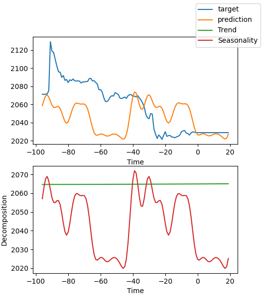
From the fig, our results look like not good enough, because we only show a rough example, and we have not carefully optimized our model, and our data key indicators are still not scientifically specified. Moreover, most of the model parameters are only used by defaults and not tuned, so we have a lot of room for optimization.

Conclusion

In this article, we discuss how to use our labeled data to predict future prices using the NBEATS model. At the same time, we also demonstrate the special interpretability decomposition function of the NBEATS model. Although our code changes are not significant, please pay attention to our discussion about covariates in the text. If you really understand the usage of different covariates, you can extend this model to other different application scenarios! I believe this will greatly help you improve the accuracy of EA and accurately complete the tasks you need to complete. Of course, this article is just an example. If you want to apply it to actual trading, it is still a bit rough. There are many places that need further optimization, so don’t use it directly in trading! At the same time, we also mentioned some information about external variables. I don’t know if anyone is interested in this direction. If I can get enough information, I may discuss how to implement it in this series of articles in the future.

So, this article ends here, I hope you can gain something!

All the code:

# Copyright 2021, MetaQuotes Ltd.
# https://www.mql5.com



import lightning.pytorch as pl
import os
from lightning.pytorch.callbacks import EarlyStopping,ModelCheckpoint
import matplotlib.pyplot as plt
import pandas as pd
from pytorch_forecasting import TimeSeriesDataSet,NBeats
from pytorch_forecasting.data import NaNLabelEncoder
from pytorch_forecasting.data.samplers import TimeSynchronizedBatchSampler
from lightning.pytorch.tuner import Tuner
import MetaTrader5 as mt
import warnings
import json


from torch.utils.data import DataLoader
from torch.utils.data.sampler import Sampler,SequentialSampler

class New_TmSrDt(TimeSeriesDataSet):
    '''
    rewrite dataset class
    '''
    def to_dataloader(self, train: bool = True, 
                      batch_size: int = 64, 
                      batch_sampler: Sampler | str = None, 
                      shuffle:bool=False,
                      drop_last:bool=False,
                      **kwargs) -> DataLoader:

        default_kwargs = dict(
            shuffle=shuffle,
            # drop_last=train and len(self) > batch_size,
            drop_last=drop_last, #
            collate_fn=self._collate_fn,
            batch_size=batch_size,
            batch_sampler=batch_sampler,
        )
        default_kwargs.update(kwargs)
        kwargs = default_kwargs
        # print(kwargs['drop_last'])
        if kwargs["batch_sampler"] is not None:
            sampler = kwargs["batch_sampler"]
            if isinstance(sampler, str):
                if sampler == "synchronized":
                    kwargs["batch_sampler"] = TimeSynchronizedBatchSampler(
                        SequentialSampler(self),
                        batch_size=kwargs["batch_size"],
                        shuffle=kwargs["shuffle"],
                        drop_last=kwargs["drop_last"],
                    )
                else:
                    raise ValueError(f"batch_sampler {sampler} unknown - see docstring for valid batch_sampler")
            del kwargs["batch_size"]
            del kwargs["shuffle"]
            del kwargs["drop_last"]

        return DataLoader(self,**kwargs)

def get_data(mt_data_len:int):
    if not mt.initialize():
        print('initialize() failed!') 
    else:
        print(mt.version())
        sb=mt.symbols_total()
        rts=None
        if sb > 0:
            rts=mt.copy_rates_from_pos("GOLD_micro",mt.TIMEFRAME_M15,0,mt_data_len) 
        mt.shutdown()
        # print(len(rts))
    rts_fm=pd.DataFrame(rts)
    rts_fm['time']=pd.to_datetime(rts_fm['time'], unit='s') 

    rts_fm['time_idx']= rts_fm.index%(max_encoder_length+2*max_prediction_length) 
    rts_fm['series']=rts_fm.index//(max_encoder_length+2*max_prediction_length)
    return rts_fm


def spilt_data(data:pd.DataFrame,
               t_drop_last:bool,
               t_shuffle:bool,
               v_drop_last:bool,
               v_shuffle:bool):
    training_cutoff = data["time_idx"].max() - max_prediction_length #max:95
    context_length = max_encoder_length
    prediction_length = max_prediction_length
    training = New_TmSrDt(
        data[lambda x: x.time_idx <= training_cutoff],
        time_idx="time_idx",
        target="close",
        categorical_encoders={"series":NaNLabelEncoder().fit(data.series)},
        group_ids=["series"],
        time_varying_unknown_reals=["close"],
        max_encoder_length=context_length,
        # min_encoder_length=max_encoder_length//2,
        max_prediction_length=prediction_length,
        # min_prediction_length=1,
        
    )

    validation = New_TmSrDt.from_dataset(training, 
                                         data, 
                                         min_prediction_idx=training_cutoff + 1)
    
    train_dataloader = training.to_dataloader(train=True,
                                              shuffle=t_shuffle, 
                                              drop_last=t_drop_last,
                                              batch_size=batch_size, 
                                              num_workers=0,)
    val_dataloader = validation.to_dataloader(train=False, 
                                              shuffle=v_shuffle,
                                              drop_last=v_drop_last,
                                              batch_size=batch_size, 
                                              num_workers=0)
    return train_dataloader,val_dataloader,training

def get_learning_rate():
    
    pl.seed_everything(42)
    trainer = pl.Trainer(accelerator="cpu", gradient_clip_val=0.1,logger=False)
    net = NBeats.from_dataset(
        training,
        learning_rate=3e-2,
        weight_decay=1e-2,
        backcast_loss_ratio=0.1,
        optimizer="AdamW",
    )
    res = Tuner(trainer).lr_find(
        net, train_dataloaders=t_loader, val_dataloaders=v_loader, min_lr=1e-5, max_lr=1e-1
    )
    # print(f"suggested learning rate: {res.suggestion()}")
    lr_=res.suggestion()
    return lr_
def train():
    early_stop_callback = EarlyStopping(monitor="val_loss", 
                                        min_delta=1e-4, 
                                        patience=10,  
                                        verbose=True, 
                                        mode="min")
    ck_callback=ModelCheckpoint(monitor='val_loss',
                                mode="min",
                                save_top_k=1,  
                                filename='{epoch}-{val_loss:.2f}')
    trainer = pl.Trainer(
        max_epochs=ep,
        accelerator="cpu",
        enable_model_summary=True,
        gradient_clip_val=1.0,
        callbacks=[early_stop_callback,ck_callback],
        limit_train_batches=30,
        enable_checkpointing=True,
    )
    net = NBeats.from_dataset(
        training,
        learning_rate=lr,
        log_interval=10,
        log_val_interval=1,
        weight_decay=1e-2,
        backcast_loss_ratio=0.0,
        optimizer="AdamW",
        stack_types=["trend", "seasonality"],
    )
    trainer.fit(
        net,
        train_dataloaders=t_loader,
        val_dataloaders=v_loader,
        # ckpt_path='best'
    )
    return trainer

if __name__=='__main__':
    ep=200
    __train=False
    mt_data_len=80000
    max_encoder_length = 96
    max_prediction_length = 20
    # context_length = max_encoder_length
    # prediction_length = max_prediction_length
    batch_size = 128
    info_file='results.json'
    warnings.filterwarnings("ignore")
    dt=get_data(mt_data_len=mt_data_len)
    if __train:
        # print(dt)
        # dt=get_data(mt_data_len=mt_data_len)
        t_loader,v_loader,training=spilt_data(dt,
                                              t_shuffle=False,t_drop_last=True,
                                              v_shuffle=False,v_drop_last=True)
        lr=get_learning_rate()
        # lr=3e-3
        trainer__=train()
        m_c_back=trainer__.checkpoint_callback
        m_l_back=trainer__.early_stopping_callback
        best_m_p=m_c_back.best_model_path
        best_m_l=m_l_back.best_score.item()

        # print(best_m_p)
        
        if os.path.exists(info_file):
            with open(info_file,'r+') as f1:
                last=json.load(fp=f1)
                last_best_model=last['last_best_model']
                last_best_score=last['last_best_score']
                if last_best_score > best_m_l:
                    last['last_best_model']=best_m_p
                    last['last_best_score']=best_m_l
                    json.dump(last,fp=f1)
        else:               
            with open(info_file,'w') as f2:
                json.dump(dict(last_best_model=best_m_p,last_best_score=best_m_l),fp=f2)

        best_model = NBeats.load_from_checkpoint(best_m_p)
        predictions = best_model.predict(v_loader, trainer_kwargs=dict(accelerator="cpu",logger=False), return_y=True)
        raw_predictions = best_model.predict(v_loader, mode="raw", return_x=True, trainer_kwargs=dict(accelerator="cpu",logger=False))
    
        for idx in range(10):  # plot 10 examples
            best_model.plot_prediction(raw_predictions.x, raw_predictions.output, idx=idx, add_loss_to_title=True)
        plt.show()
    else:
        with open(info_file) as f:
            best_m_p=json.load(fp=f)['last_best_model']
        print('model path is:',best_m_p)
        
        best_model = NBeats.load_from_checkpoint(best_m_p)

        offset=1
        dt=dt.iloc[-max_encoder_length-offset:-offset,:]
        last_=dt.iloc[-1] 
        # print(len(dt))
        for i in range(1,max_prediction_length+1):
            dt.loc[dt.index[-1]+1]=last_
        dt['series']=0
        # dt['time_idx']=dt.apply(lambda x:x.index,args=1)
        dt['time_idx']=dt.index-dt.index[0]
        # dt=get_data(mt_data_len=max_encoder_length)
        predictions = best_model.predict(dt, mode='raw',trainer_kwargs=dict(accelerator="cpu",logger=False),return_x=True)
        # best_model.plot_prediction(predictions.x,predictions.output,show_future_observed=False)
        best_model.plot_interpretation(predictions.x,predictions.output,idx=0)
        plt.show()