Data label for time series mining (Part 6)：Apply and Test in EA Using ONNX

MetaTrader 5 — Examples | 18 January 2024, 13:22

1 154

Yuqiang Pan

Introduction

We discussed in the previous article how to use socket (websocket) to communicate between EA and python server to solve the backtesting problem, and also discussed why we adopted this technique. In this article, we will discuss how to use onnx, which is natively supported by mql5, to perform inference with our model, but this method has some limitations. If your model uses operators that are not supported by onnx, it may end in failure, so this method is not suitable for all models (of course, you can also add operators to support your model, but it requires a lot of time and effort). This is why I spent a lot of space in the previous article to introduce the socket method and recommend it to you.

Of course, converting a general model to onnx format is very convenient, and it provides us with effective support for cross-platform operations. This article mainly involves some basic operations of operating ONNX models in mql5, including how to match the input and output of torch models and ONNX models, and how to convert suitable data formats for ONNX models. Of course, it also includes EA order management. I will explain it in detail for you. Now let’s start the main topic of this article!

Table of contents:

Directory Structure

When we perform model conversion, we will involve reading the model and configuration files, but embarrassingly, I found that I did not introduce the directory structure of the script in the previous articles, which may cause you to not find the location of your model and configuration files. So we sort out the directory structure of our script here. When we use lightning-pytorch to train the model, we did not define the model save location in the callbacks (the callbacks responsible for managing the model Checkpoint are the ModelCheckpoint class), only defined the model name, so the trainer will save the model in the default path.

    ck_callback=ModelCheckpoint(monitor='val_loss',
                                mode="min",
                                save_top_k=1,  
                                filename='{epoch}-{val_loss:.2f}')

At this time, the trainer will save the model in the root directory, which may be a bit vague, so I use a few pictures to illustrate, this will make you very clear about what files are saved during the training process and where the files are.

First of all, our model save location, this path contains different version folders, each version folder contains checkpoints folder, events file, parameter file, in the checkpoints folder contains the model file we saved:

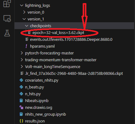
When training the model, we used a model to find the best learning rate, which will be saved in the root directory of the folder:

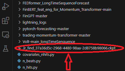
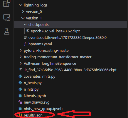
When training, we will save a results.json file to record the best model path and the best score, which will be used when we load the model, it is saved in the root directory of the folder:

Convert Torch Model to ONNX Model

We still use the NBeats model as an example. The following code will be mainly added in the inference part of Nbeats.py. This script was created when I introduced the NBeats model in the previous article. Due to the special nature of the NBeats model, it may be difficult to export the ONNX model using the general method. You need to debug the inference process of the model and then get the relevant information from it to define the relevant parameters required for export. But I have done this process for you, so don’t worry, just follow the steps in the article step by step, and all the problems will be easily solved.

1. Install the required libraries

Before converting the model, there is another important step to do, which is to install the relevant libraries of ONNX. If you only export the model, you only need to install the onnx library: pip install onnx. But since we also need to test the model after converting it, we also need to install the onnxruntime library. This library is divided into two versions: cpu runtime and GPU runtime. If the model is large and complex, you may need to install the GPU version to speed up the inference process. Since our model only needs cpu inference, the GPU acceleration effect is not obvious, so I recommend installing the CPU version: pip install onnxruntime.

2. Get input information

First, you need to switch the model from training mode to inference mode: best_model.eval(). The reason for doing this is that the model’s training mode and inference mode are different, and we only need the model’s inference mode, which will reduce the complexity of the model and only retain the input required for inference. Then we need to create a Dataloader after loading the data to get the complete input items, get an iterator from this Dataloader object, and then call the next function to get the first batch of data. The first element contains all the input information we need. During the export process of the model, torch will automatically select the required input items for us. Now we use the spilt_data() function that has been defined before to directly create a Dataloader after loading the data: t_loader,v_loader,training=spilt_data(dt,t_shuffle=False,t_drop_last=True,v_shuffle=False,v_drop_last=True) Create a dictionary to store the input required for exporting the model: input_dict = {} Get all the input objects, here we use v_loader to get them, because we need the inference process: items = next(iter(v_loader))[0] Create a list to store all the input names: input_names=[] Then we iterate through the items to get all the inputs and input names:

for item in items:
            input_dict[item] = items[item][-1:]
            # print("{}:{}".format(item,input_dict[item].shape()))
            input_names.append(item)

3. Getting output information

Before getting the output, we need to run an inference first, and then get the output information we need from the inference result. This is the original inference process:

offset=1
dt=dt.iloc[-max_encoder_length-offset:-offset,:]
last_=dt.iloc[-1] 
# print(len(dt))
for i in range(1,max_prediction_length+1):
    dt.loc[dt.index[-1]+1]=last_
dt['series']=0
# dt['time_idx']=dt.apply(lambda x:x.index,args=1)
dt['time_idx']=dt.index-dt.index[0]
input_=dt.loc[:,['close','series','time_idx']]
predictions = best_model.predict(input_, mode='raw',trainer_kwargs=dict(accelerator="cpu",logger=False),return_x=True)

The inference information is in the output of the predictions object, we iterate through this object to get all the output information, so we add the following statement here:

output_names=[]
for out in predictions.output._fields:
    output_names.append(out)

4. Exporting the model

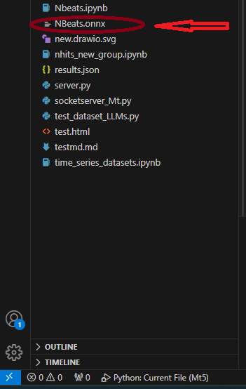
First, we define the input_sample required for exporting the model: input_1=(input_dict,{}) , don’t ask why, just do it! Then we use the to_onnx() method in the NBeats class to export to ONNX, which also requires a file path parameter, we directly export to the root directory, named “NBeats.onnx”: best_model.to_onnx(file_path=‘NBeats.onnx’, input_sample=input_1, input_names=input_names, output_names=output_names). After the program runs to this point, we will find the “NBeats.onnx” file in the root directory of the current folder:

Note:

1. Because if the input name is not complete, the export model will automatically name it when exporting, which will cause some confusion, making us not know which one is the real input, so we choose to input all the names to the export function to ensure the consistency of the input names of the exported model.

2. In the Dataloader, the input data includes “encoder_cat”, “encoder_cont” and other multiple inputs generated by the encoder and decoder, while in the inference process we only need “encoder_cont” and “target_scale” two. So don’t think that the step of matching the input data is redundant, in some models that require encoders and decoders, this step is necessary. 3. The environment configuration used by the author during the test process: python-3.10;ONNX version-8; pytorch-2.1.1;operators-17.

Testing the Converted Model

In the previous part, we have successfully exported the torch model as an ONNX model. The next important task is to test this model and see if the output of this model is the same as the original model. This is very important, because during the export process, some operators may have deviations due to the torch version and the onnx runtime kernel compatibility issues. In this case, manual intervention may be required when exporting the model.

First, import the ONNX runtime library: import onnxruntime as ort.
Load the model file “NBeats.onnx”: sess = ort.InferenceSession(“NBeats.onnx”).
Get the input names of the ONNX model by iterating over the return value of sess.get_inputs(), which are used to match the input data: input_names = [input.name for input in sess.get_inputs()].
We don’t need to compare all the outputs, so we only get the first item of the output to compare and see if the results are the same: output_name = sess.get_outputs()[0].name.
To compare whether the results are the same, the input must be the same, so the model input must be consistent with the data used for inference. But we need to convert it to Dataloader format first and use input_names to match the input data, because not all the inputs will be loaded during the inference process. First, load the input data as time series data using the from_parameters() method of the TimeSeriesDataSet class: input_ds = New_TmSrDt.from_parameters(best_model.dataset_parameters, input_,predict=True). Then convert it to Dataloader type using the to_dataloader() class method: input_dl = input_ds.to_dataloader(train=False, batch_size=1, num_workers=0).
Match the input data. First, we need to get a batch of data and take out the first element: input_dict = next(iter(input_dl))[0]. Then use input_names to match the input data required by the input: input_data = [input_dict[name].numpy() for name in input_names]
Run the inference: pred_onnx = sess.run([output_name], dict(zip(input_names, input_data)))[0].
Print the torch inference result and the onnx inference result and compare them.

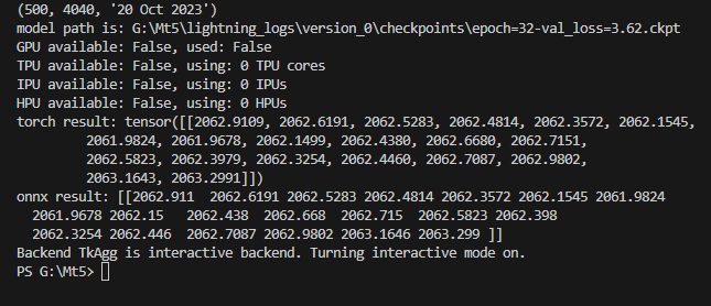
Now, print the torch inference result:

torch result: tensor([[2062.9109, 2062.6191, 2062.5283, 2062.4814, 2062.3572, 2062.1545, 2061.9824, 2061.9678, 2062.1499, 2062.4380, 2062.6680, 2062.7151, 2062.5823, 2062.3979, 2062.3254, 2062.4460, 2062.7087, 2062.9802, 2063.1643, 2063.2991]])

Print the onnx inference result:

onnx result: [[2062.911 2062.6191 2062.5283 2062.4814 2062.3572 2062.1545 2061.9824 2061.9678 2062.15 2062.438 2062.668 2062.715 2062.5823 2062.398 2062.3254 2062.446 2062.7087 2062.9802 2063.1646 2063.299 ]]

We can see that our model inference results are the same. The next step is to configure the exported model in mql5. As shown in the figure:

Complete code:

# Copyright 2021, MetaQuotes Ltd.
# https://www.mql5.com



import lightning.pytorch as pl
import os
from lightning.pytorch.callbacks import EarlyStopping,ModelCheckpoint
import matplotlib.pyplot as plt
import pandas as pd
from pytorch_forecasting import TimeSeriesDataSet,NBeats
from pytorch_forecasting.data import NaNLabelEncoder
from pytorch_forecasting.data.samplers import TimeSynchronizedBatchSampler
from lightning.pytorch.tuner import Tuner
import MetaTrader5 as mt
import warnings
import json

from torch.utils.data import DataLoader
from torch.utils.data.sampler import Sampler,SequentialSampler

class New_TmSrDt(TimeSeriesDataSet):
    '''
    rewrite dataset class
    '''
    def to_dataloader(self, train: bool = True, 
                      batch_size: int = 64, 
                      batch_sampler: Sampler | str = None, 
                      shuffle:bool=False,
                      drop_last:bool=False,
                      **kwargs) -> DataLoader:

        default_kwargs = dict(
            shuffle=shuffle,
            # drop_last=train and len(self) > batch_size,
            drop_last=drop_last, #
            collate_fn=self._collate_fn,
            batch_size=batch_size,
            batch_sampler=batch_sampler,
        )
        default_kwargs.update(kwargs)
        kwargs = default_kwargs
        # print(kwargs['drop_last'])
        if kwargs["batch_sampler"] is not None:
            sampler = kwargs["batch_sampler"]
            if isinstance(sampler, str):
                if sampler == "synchronized":
                    kwargs["batch_sampler"] = TimeSynchronizedBatchSampler(
                        SequentialSampler(self),
                        batch_size=kwargs["batch_size"],
                        shuffle=kwargs["shuffle"],
                        drop_last=kwargs["drop_last"],
                    )
                else:
                    raise ValueError(f"batch_sampler {sampler} unknown - see docstring for valid batch_sampler")
            del kwargs["batch_size"]
            del kwargs["shuffle"]
            del kwargs["drop_last"]

        return DataLoader(self,**kwargs)

def get_data(mt_data_len:int):
    if not mt.initialize():
        print('initialize() failed!') 
    else:
        print(mt.version())
        sb=mt.symbols_total()
        rts=None
        if sb > 0:
            rts=mt.copy_rates_from_pos("GOLD_micro",mt.TIMEFRAME_M15,0,mt_data_len) 
        mt.shutdown()
        # print(len(rts))
    rts_fm=pd.DataFrame(rts)
    rts_fm['time']=pd.to_datetime(rts_fm['time'], unit='s') 

    rts_fm['time_idx']= rts_fm.index%(max_encoder_length+2*max_prediction_length) 
    rts_fm['series']=rts_fm.index//(max_encoder_length+2*max_prediction_length)
    return rts_fm


def spilt_data(data:pd.DataFrame,
               t_drop_last:bool,
               t_shuffle:bool,
               v_drop_last:bool,
               v_shuffle:bool):
    training_cutoff = data["time_idx"].max() - max_prediction_length #max:95
    context_length = max_encoder_length
    prediction_length = max_prediction_length
    training = New_TmSrDt(
        data[lambda x: x.time_idx <= training_cutoff],
        time_idx="time_idx",
        target="close",
        categorical_encoders={"series":NaNLabelEncoder().fit(data.series)},
        group_ids=["series"],
        time_varying_unknown_reals=["close"],
        max_encoder_length=context_length,
        # min_encoder_length=max_encoder_length//2,
        max_prediction_length=prediction_length,
        # min_prediction_length=1,
        
    )

    validation = New_TmSrDt.from_dataset(training, 
                                         data, 
                                         min_prediction_idx=training_cutoff + 1)
    
    train_dataloader = training.to_dataloader(train=True,
                                              shuffle=t_shuffle, 
                                              drop_last=t_drop_last,
                                              batch_size=batch_size, 
                                              num_workers=0,)
    val_dataloader = validation.to_dataloader(train=False, 
                                              shuffle=v_shuffle,
                                              drop_last=v_drop_last,
                                              batch_size=batch_size, 
                                              num_workers=0)
    return train_dataloader,val_dataloader,training

def get_learning_rate():
    
    pl.seed_everything(42)
    trainer = pl.Trainer(accelerator="cpu", gradient_clip_val=0.1,logger=False)
    net = NBeats.from_dataset(
        training,
        learning_rate=3e-2,
        weight_decay=1e-2,
        backcast_loss_ratio=0.1,
        optimizer="AdamW",
    )
    res = Tuner(trainer).lr_find(
        net, train_dataloaders=t_loader, val_dataloaders=v_loader, min_lr=1e-5, max_lr=1e-1
    )
    # print(f"suggested learning rate: {res.suggestion()}")
    lr_=res.suggestion()
    return lr_
def train():
    early_stop_callback = EarlyStopping(monitor="val_loss", 
                                        min_delta=1e-4, 
                                        patience=10,  
                                        verbose=True, 
                                        mode="min")
    ck_callback=ModelCheckpoint(monitor='val_loss',
                                mode="min",
                                save_top_k=1,  
                                filename='{epoch}-{val_loss:.2f}')
    trainer = pl.Trainer(
        max_epochs=ep,
        accelerator="cpu",
        enable_model_summary=True,
        gradient_clip_val=1.0,
        callbacks=[early_stop_callback,ck_callback],
        limit_train_batches=30,
        enable_checkpointing=True,
    )
    net = NBeats.from_dataset(
        training,
        learning_rate=lr,
        log_interval=10,
        log_val_interval=1,
        weight_decay=1e-2,
        backcast_loss_ratio=0.0,
        optimizer="AdamW",
        stack_types=["trend", "seasonality"],
    )
    trainer.fit(
        net,
        train_dataloaders=t_loader,
        val_dataloaders=v_loader,
        # ckpt_path='best'
    )
    return trainer

if __name__=='__main__':
    ep=200
    __train=False
    mt_data_len=80000
    max_encoder_length = 96
    max_prediction_length = 20
    # context_length = max_encoder_length
    # prediction_length = max_prediction_length
    batch_size = 128
    info_file='results.json'
    warnings.filterwarnings("ignore")
    dt=get_data(mt_data_len=mt_data_len)
    if __train:
        # print(dt)
        # dt=get_data(mt_data_len=mt_data_len)
        t_loader,v_loader,training=spilt_data(dt,
                                              t_shuffle=False,t_drop_last=True,
                                              v_shuffle=False,v_drop_last=True)
        lr=get_learning_rate()
        # lr=3e-3
        trainer__=train()
        m_c_back=trainer__.checkpoint_callback
        m_l_back=trainer__.early_stopping_callback
        best_m_p=m_c_back.best_model_path
        best_m_l=m_l_back.best_score.item()

        # print(best_m_p)
        
        if os.path.exists(info_file):
            with open(info_file,'r+') as f1:
                last=json.load(fp=f1)
                last_best_model=last['last_best_model']
                last_best_score=last['last_best_score']
                if last_best_score > best_m_l:
                    last['last_best_model']=best_m_p
                    last['last_best_score']=best_m_l
                    json.dump(last,fp=f1)
        else:               
            with open(info_file,'w') as f2:
                json.dump(dict(last_best_model=best_m_p,last_best_score=best_m_l),fp=f2)

        best_model = NBeats.load_from_checkpoint(best_m_p)
        predictions = best_model.predict(v_loader, trainer_kwargs=dict(accelerator="cpu",logger=False), return_y=True)
        raw_predictions = best_model.predict(v_loader, mode="raw", return_x=True, trainer_kwargs=dict(accelerator="cpu",logger=False))
    
        for idx in range(10):  # plot 10 examples
            best_model.plot_prediction(raw_predictions.x, raw_predictions.output, idx=idx, add_loss_to_title=True)
        plt.show()
    else:
        with open(info_file) as f:
            best_m_p=json.load(fp=f)['last_best_model']
        print('model path is:',best_m_p)
        best_model = NBeats.load_from_checkpoint(best_m_p)

        # added for input
        best_model.eval()
        t_loader,v_loader,training=spilt_data(dt,
                                t_shuffle=False,t_drop_last=True,
                                v_shuffle=False,v_drop_last=True)

        input_dict = {}
        items = next(iter(v_loader))[0]
        input_names=[]
        for item in items:
            input_dict[item] = items[item][-1:]
            # print("{}:{}".format(item,input_dict[item].shape()))
            input_names.append(item)  
# ------------------------eval----------------------------------------------

        offset=1
        dt=dt.iloc[-max_encoder_length-offset:-offset,:]
        last_=dt.iloc[-1] 
        # print(len(dt))
        for i in range(1,max_prediction_length+1):
            dt.loc[dt.index[-1]+1]=last_
        dt['series']=0
        # dt['time_idx']=dt.apply(lambda x:x.index,args=1)
        dt['time_idx']=dt.index-dt.index[0]
        input_=dt.loc[:,['close','series','time_idx']]
        predictions = best_model.predict(input_, mode='raw',trainer_kwargs=dict(accelerator="cpu",logger=False),return_x=True)
        
        output_names=[]
        for out in predictions.output._fields:
            output_names.append(out)  
# ----------------------------------------------------------------------------
        
        input_1=(input_dict,{}) 
        best_model.to_onnx(file_path='NBeats.onnx', 
                           input_sample=input_1, 
                           input_names=input_names,
                           output_names=output_names)

        import onnxruntime as ort
        sess = ort.InferenceSession("NBeats.onnx")
        input_names = [input.name for input in sess.get_inputs()]
        # for input in sess.get_inputs():
        #     print(input.name,':',input.shape) 
        output_name = sess.get_outputs()[0].name

# ------------------------------------------------------------------------------
        input_ds = New_TmSrDt.from_parameters(best_model.dataset_parameters, input_,predict=True)
        input_dl = input_ds.to_dataloader(train=False, batch_size=1, num_workers=0)
        input_dict = next(iter(input_dl))[0]
        input_data = [input_dict[name].numpy() for name in input_names]
        pred_onnx = sess.run([output_name], dict(zip(input_names, input_data)))
        print("torch result:",predictions.output[0])
        print("onnx result:",pred_onnx[0])
# -------------------------------------------------------------------------------
        
        
        best_model.plot_interpretation(predictions.x,predictions.output,idx=0)
        plt.show()

Create EA with ONNX Model

We have completed the model conversion and testing, and now we will create an expert file named onnx.mq5. In EA, we plan to use OnTimer() to manage the inference logic of the model, and use OnTick() to manage the order logic, so that we can set how often to run the inference, instead of running the inference every time a quote comes, which will cause serious resource occupation. Similarly, in this EA, we will not provide complex trading logic, just provide a demonstration example, please do not directly use this EA for trading!

1. View the ONNX model structure

This step is very important, we need to define the input and output for the ONNX model in EA, so we need to view the model structure, to determine the number, data type and data dimension of the input and output. To view the ONNX model, you can open it directly in the mql5 editor, and you will see the model structure. It will also give you the input and output styles, but it is not editable. We can also use Netron or WinML Dashboard tools, the tool we use in this article is Netron.

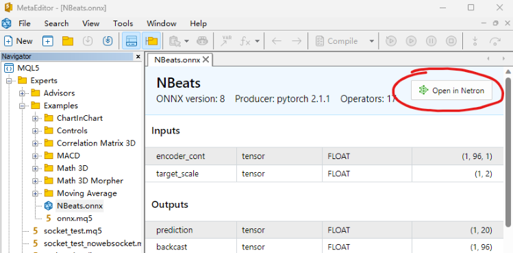
We find our model file "NBeats.onnx" in the mql5 IDE and open it directly, in the annotation position below you can find the "Open in Netron" option, click the button and the model file will be opened automatically.

Or right-click on our model file in the IDE's file explorer and you will see the "Open in Netron" option.

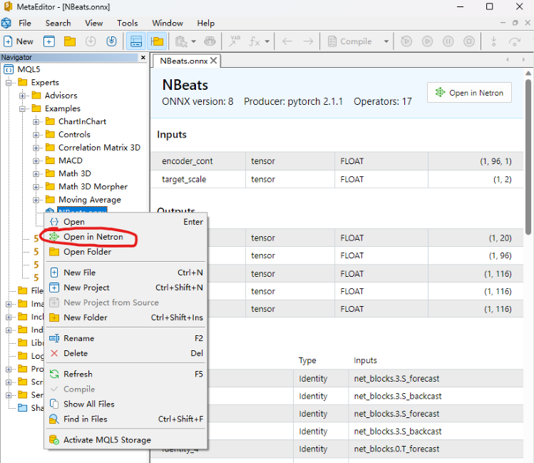
If you don’t have Netron tool, the IDE will guide you to install it.

The model looks like this after opening:

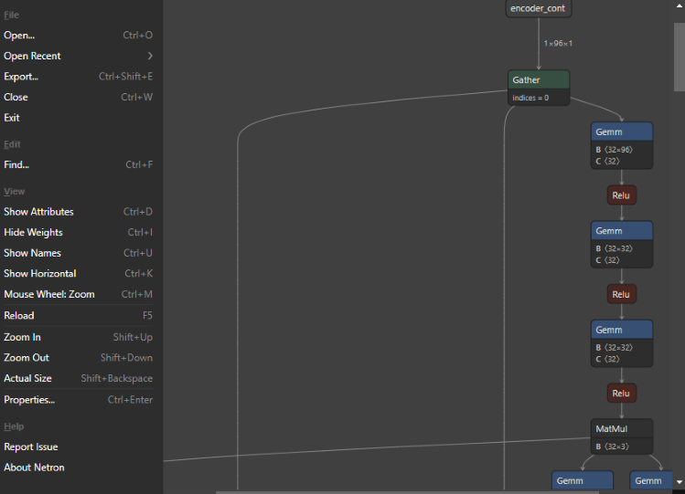
You can see that the whole interface is very simple and refreshing, and the function is very powerful. We can even use it to edit the model nodes. Now back to the topic, we click on the first node, and Netron will show us the relevant information of the model:

inf

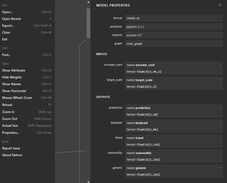
You can see that the format of the exported NBeats model is: ONNX v8, pytorch version is: pytorch 2.1.1, export tool is: ai.onnx v17.

There are two inputs, the first one is: encoder_cont, dimension is: [1,96,1], data format is: float32; the second one is: target_scale, dimension is: [1,2], data format is: float32.

There are five outputs, the first one is: prediction, dimension is: [1,20]; the second one is: backcast, dimension is: [1,96]; the other three interpretable outputs trend, seasonality, generic dimension are [1,116]. All output data formats are float32.

2. Define the input and output of the model

We already know the input and output format of the model, and the input and output formats supported by onnx in mql5 are arrays, matrices and vectors. Now let’s define them in EA. First, define the input in OnTimer(), both are arrays:

The first input: matrixf in_normf;
The second input: float in1[1][2];

Because we need to call the output results of the model in OnTick(), it is unreasonable to define the output of the model in OnTimer(), and they need to be defined as global variables. The model inference results and the model loading handle also need to be defined as global variables:

Model handle: long handle;
The first inference result: vectorf y=vector<float>::Zeros(20);
The second inference result: vectorf backcast=vector<float>::Zeros(96);
The third inference result: vectorf trend=vector<float>::Zeros(116);
The fourth inference result: vectorf seasonality=vector<float>::Zeros(116);
The fifth inference result: vectorf generic=vector<float>::Zeros(116);
Define the prediction result: string pre=NULL;

3. Define the inference logic

Ⅰ Initialization

First, import the ONNX model as an external resource in EA: #resource “NBeats.onnx” as uchar ExtModel[]. Initialize the Timer in the OnInit() function: EventSetTimer(300), this value can be set by yourself. Load the model and get the model handle: handle=OnnxCreateFromBuffer(ExtModel,ONNX_DEBUG_LOGS). If you want to view the input or output information of the model, you can add the following statement:

   long in_ct=OnnxGetInputCount(handle);
   OnnxTypeInfo inf;
   for(int i=0;i<in_ct;i++){
   
   Print(OnnxGetInputName(handle,i));
   bool re=OnnxGetInputTypeInfo(handle,i,inf);
   //Print("map:",inf.map,"seq:",inf.sequence,"tensor:",inf.tensor,"type:",inf.type);
   Print(re,GetLastError());
   }

Ⅱ Data Processing

We have already defined the input and output of the model before, and next we need to know the specific definition of these variables, what kind of data they are. This requires us to find their definitions in the timeseries.py file in the pytorch_forecasting library. This article will not explain this file in detail, let’s reveal the answer directly.

The first input:

"encoder_cont" is actually the normalized value of the target variable, of course pytorch_forecasting provides different methods EncoderNormalizer, GroupNormalizer, MultiNormalizer, NaNLabelEncoder, TorchNormalizer, these methods may be difficult to implement in mql5, so in this article we directly use the ordinary normalize method. First define an empty MqlRates: MqlRates rates[], and then use it to copy the last 96 bars of close values: if(!CopyRates(_Symbol,_Period,0,96,rates)) return, if the copy fails, return directly. We also need to define a matrix to receive this value, which is used to calculate the mean and variance: matrix in0_m(96,1). Copy the close value of this rate to the in0_m matrix: for(int i=0; i<96; i++) in0_m[i][0]= rates[i].close. Calculate the mean: vector m=in0_m.Mean(0); calculate the variance: vector s=in0_m.Std(0). Create a matrix mm to store the mean: matrix mm(96,1); create a matrix ms to store the variance: matrix ms(96,1). Copy the mean and variance to the auxiliary matrix:

    for(int i=0; i<96; i++) 
     { 
        mm.Row(m,i); 
        ms.Row(s,i); 
         }

Now we calculate the normalized matrix, first subtract the mean: in0_m-=mm, then divide by the standard deviation: in0_m/=ms, and then copy the matrix to the input matrix and convert the data type to float: in_normf.Assign(in0_m)

The second input:

"target_scale" is actually the scaling range of the target variable, its first value is actually the mean of the target variable: in1[0][0]=m[0], the second data is the variance of the target variable: in1[0][1]=s[0]

Ⅲ Run Inference

When running ONNX model inference, the input and output displayed in the model structure must be all defined, no one can be missing, even if some inputs you do not need must also be passed as parameters to the OnnxRun() function, this is very important, otherwise it will definitely report an error.

   if(!OnnxRun(handle,
      ONNX_DEBUG_LOGS | ONNX_NO_CONVERSION,
      in_normf,
      in1,
      y,
      backcast,
      trend,
      seasonality,
      generic)) 
    { 
      Print("OnnxRun failed, error ",GetLastError()); 
      OnnxRelease(handle);
      return; 
      }

4. Inference Results

We make a simple assumption: if the mean of the predicted value is greater than the average of the highest and lowest values of the current bar, we assume that the future will be an upward trend, and set pre to “buy”, otherwise set pre to “sell”:

   if (y.Mean()>iHigh(_Symbol,_Period,0)/2+iLow(_Symbol,_Period,0)/2)
      pre="buy";
   else
      pre="sell";

5. Order Processing Logic

This part we have already introduced in detail in the article Data label for time series mining(Part 5)：Apply and Test in EA Using Socket, this article will not do a detailed introduction, we only need to copy the main logic to OnTick() and use it directly. It should be noted that after each execution, pre is set to NULL, and during the prediction process we will assign values to these two values, which ensures the synchronization of the order operation process and the prediction process, and will not be affected by the previous prediction value. This step is very important, otherwise it will cause some logical confusion, the following is the complete order processing code:

void OnTick()
  {
//---
   MqlTradeRequest request;
   MqlTradeResult result;
   //int x=SymbolInfoInteger(_Symbol,SYMBOL_FILLING_MODE);

    if (pre!=NULL)
    {
        //Print("The predicted value is:",pre);
        ulong numt=0;
        ulong tik=0;
        bool sod=false;
        ulong tpt=-1;
        ZeroMemory(request); 
        numt=PositionsTotal();
        //Print("All tickets: ",numt);
        if (numt>0)
         {  tik=PositionGetTicket(numt-1);    
            sod=PositionSelectByTicket(tik);
            tpt=PositionGetInteger(POSITION_TYPE);//ORDER_TYPE_BUY or ORDER_TYPE_SELL
            if (tik==0 || sod==false || tpt==0) return; 
            }
        if (pre=="buy")
        {  
           
           if (tpt==POSITION_TYPE_BUY)
               return;
               
            request.action=TRADE_ACTION_DEAL;
            request.symbol=Symbol();
            request.volume=0.1;
            request.deviation=5;
            request.type_filling=ORDER_FILLING_IOC;
            request.type = ORDER_TYPE_BUY;  
            request.price = SymbolInfoDouble(Symbol(), SYMBOL_ASK);
           if(tpt==POSITION_TYPE_SELL)
             {
               request.position=tik;
               Print("Close sell order.");
                    }
           else{     
  
            Print("Open buy order.");
                     }
            OrderSend(request, result);
               }
        else{
           if (tpt==POSITION_TYPE_SELL)
               return;
               
            request.action = TRADE_ACTION_DEAL;      
            request.symbol = Symbol();  
            request.volume = 0.1;  
            request.type = ORDER_TYPE_SELL;  
            request.price = SymbolInfoDouble(Symbol(), SYMBOL_BID);  
            request.deviation = 5; 
            //request.type_filling=SymbolInfoInteger(_Symbol,SYMBOL_FILLING_MODE);
            request.type_filling=ORDER_FILLING_IOC;
           if(tpt==POSITION_TYPE_BUY)
               {
               request.position=tik;
               Print("Close buy order.");
                    }
           else{

               Print("OPen sell order.");
                    }
            
            OrderSend(request, result);
              }
        //is_pre=false;
        }
    pre=NULL;

  }

6. Recycle Resources

When the EA runs, we need to close the timer and release the ONNX model instance handle, so we need to add the following code to the OnDeinit(const int reason) function:

void OnDeinit(const int reason)
  {
//---
   //— destroy timer 
  EventKillTimer(); 
  //— complete operation 
  OnnxRelease(handle); 
  }

Here we have basically finished writing the code, and then we need to load and test the EA in the backtest.

Note:

1. When setting the input and output of the ONNX model, you need to pay attention to the data format matching.

2. We only use the first predicted value of the output here, which does not mean that other outputs have no value. In the article “Data label for time series mining (Part 4)：Interpretability Decomposition Using Label Data” of this series, we introduced the interpretability of the NBeats model, which is implemented using other outputs. We have already checked their visualization with python, and we will not add the visualization function in EA in this article. Readers who are interested can try to add one or more of them to the chart for visualization.

Backtesting

Before starting the backtesting, there is one thing to note: our ONNX model must be placed in the same directory as the onnx.mq5 file, otherwise it will fail to load the model file! Everything is ready, now open the mql5 editor, click the compile button, and generate the compiled file. If it compiles smoothly, press Ctrl+F5 to start the backtesting in debug mode. A new window will open to show the testing process. My output log:

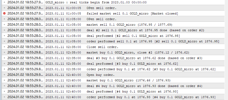
Backtesting results:

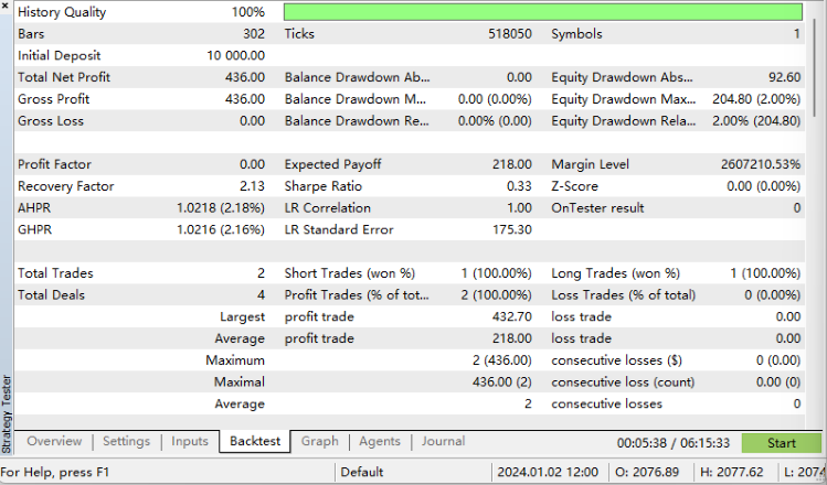
We did it！

Complete code:

//+------------------------------------------------------------------+
//|                                                         onnx.mq5 |
//|                                  Copyright 2023, MetaQuotes Ltd. |
//|                                             https://www.mql5.com |
//+------------------------------------------------------------------+
#property copyright "Copyright 2023, MetaQuotes Ltd."
#property link      "https://www.mql5.com"
#property version   "1.00"

#resource "NBeats.onnx" as uchar ExtModel[] 



long handle;
vectorf y=vector<float>::Zeros(20); 
vectorf backcast=vector<float>::Zeros(96);
vectorf trend=vector<float>::Zeros(116);
vectorf seasonality=vector<float>::Zeros(116);
vectorf generic=vector<float>::Zeros(116);
//bool is_pre=false;
string pre=NULL;

//+------------------------------------------------------------------+
//| Expert initialization function                                   |
//+------------------------------------------------------------------+
int OnInit()
  {
//---
   EventSetTimer(300); 
   handle=OnnxCreateFromBuffer(ExtModel,ONNX_DEBUG_LOGS); 
   //— specify the shape of the input data 

   long in_ct=OnnxGetInputCount(handle);
   OnnxTypeInfo inf;
   for(int i=0;i<in_ct;i++){
   
   Print(OnnxGetInputName(handle,i));
   bool re=OnnxGetInputTypeInfo(handle,i,inf);
   //Print("map:",inf.map,"seq:",inf.sequence,"tensor:",inf.tensor,"type:",inf.type);
   Print(re,GetLastError());
   }
   //long in_nm=OnnxGetInputName()
   
   


//— return initialization result 
 
//---
   return(INIT_SUCCEEDED);
  }
//+------------------------------------------------------------------+
//| Expert deinitialization function                                 |
//+------------------------------------------------------------------+
void OnDeinit(const int reason)
  {
//---
   //— destroy timer 
  EventKillTimer(); 
  //— complete operation 
  OnnxRelease(handle); 
  }
//+------------------------------------------------------------------+
//| Expert tick function                                             |
//+------------------------------------------------------------------+
void OnTick()
  {
//---
   MqlTradeRequest request;
   MqlTradeResult result;
   //int x=SymbolInfoInteger(_Symbol,SYMBOL_FILLING_MODE);

    if (pre!=NULL)
    {
        //Print("The predicted value is:",pre);
        ulong numt=0;
        ulong tik=0;
        bool sod=false;
        ulong tpt=-1;
        ZeroMemory(request); 
        numt=PositionsTotal();
        //Print("All tickets: ",numt);
        if (numt>0)
         {  tik=PositionGetTicket(numt-1);    
            sod=PositionSelectByTicket(tik);
            tpt=PositionGetInteger(POSITION_TYPE);//ORDER_TYPE_BUY or ORDER_TYPE_SELL
            if (tik==0 || sod==false || tpt==0) return; 
            }
        if (pre=="buy")
        {  
           
           if (tpt==POSITION_TYPE_BUY)
               return;
               
            request.action=TRADE_ACTION_DEAL;
            request.symbol=Symbol();
            request.volume=0.1;
            request.deviation=5;
            request.type_filling=ORDER_FILLING_IOC;
            request.type = ORDER_TYPE_BUY;  
            request.price = SymbolInfoDouble(Symbol(), SYMBOL_ASK);
           if(tpt==POSITION_TYPE_SELL)
             {
               request.position=tik;
               Print("Close sell order.");
                    }
           else{     
  
            Print("Open buy order.");
                     }
            OrderSend(request, result);
               }
        else{
           if (tpt==POSITION_TYPE_SELL)
               return;
               
            request.action = TRADE_ACTION_DEAL;      
            request.symbol = Symbol();  
            request.volume = 0.1;  
            request.type = ORDER_TYPE_SELL;  
            request.price = SymbolInfoDouble(Symbol(), SYMBOL_BID);  
            request.deviation = 5; 
            //request.type_filling=SymbolInfoInteger(_Symbol,SYMBOL_FILLING_MODE);
            request.type_filling=ORDER_FILLING_IOC;
           if(tpt==POSITION_TYPE_BUY)
               {
               request.position=tik;
               Print("Close buy order.");
                    }
           else{

               Print("OPen sell order.");
                    }
            
            OrderSend(request, result);
              }
        //is_pre=false;
        }
    pre=NULL;

  }
//+------------------------------------------------------------------+
void OnTimer() 
{ 
   //float in0[1][96][1];
   matrixf in_normf; 
   float in1[1][2];
//— get the last 10 bars 
   MqlRates rates[]; 
   if(!CopyRates(_Symbol,_Period,0,96,rates)) return; 
  //— input a set of OHLC vectors 


   //double out[1][20];
   matrix in0_m(96,1);
   for(int i=0; i<96; i++) 
     { 
       in0_m[i][0]= rates[i].close;
       } 
   //— normalize the input data 
   // matrix x_norm=x; 
    vector m=in0_m.Mean(0);  
    vector s=in0_m.Std(0); 
    
    in1[0][0]=m[0];
    in1[0][1]=s[0];
    matrix mm(96,1); 
    matrix ms(96,1); 
   //    //— fill in the normalization matrices 
    for(int i=0; i<96; i++) 
     { 
        mm.Row(m,i);  
        ms.Row(s,i); 
         } 
   //    //— normalize the input data 
   in0_m-=mm;  
   in0_m/=ms; 
   // //— convert normalized input data to float type 
   
   in_normf.Assign(in0_m); 
    //— get the output data of the model here, i.e. the price prediction 
    
    //— run the model 
   if(!OnnxRun(handle,
      ONNX_DEBUG_LOGS | ONNX_NO_CONVERSION,
      in_normf,
      in1,
      y,
      backcast,
      trend,
      seasonality,
      generic)) 
    { 
      Print("OnnxRun failed, error ",GetLastError()); 
      OnnxRelease(handle);
      return; 
      } 
    //— print the output value of the model to the log 
   //Print(y); 
   //is_pre=true;
   if (y.Mean()>iHigh(_Symbol,_Period,0)/2+iLow(_Symbol,_Period,0)/2)
      pre="buy";
   else
      pre="sell";
}

Summary

This article is expected to be the last one in this series. In this article, we have introduced the whole process of converting a torch model to an ONNX model in detail, including how to find the input and output of the model, how to define their formats, how to match them with the model, and some data processing techniques. The difficulty of this article lies in how to export a model with complex input and output as an ONNX model. We hope that readers can get inspiration and gain from it! Of course, our test EA still has a lot of room for improvement. For example, you can visualize the trend and seasonality of the NBeats model output in the chart, or use the output trend to judge the order direction, etc.

There are countless possibilities as long as you do it. The example in the article is just a simplest example, but the core content is relatively complete. You can freely expand and use it, but please note that do not use this EA for real trading casually! This series of articles provides a variety of and relatively complete solutions from making data sets to training different time series prediction models, and then to how to use them in backtesting. Even beginners can complete the whole process step by step and apply it to practice, so this series can end successfully!
Thank you for reading, I hope you have learned something, and have a nice day!

Attached files |

Download ZIP

NBeats.onnx (6949.02 KB)

onnx.mq5 (11.99 KB)

n_beats.py (11.07 KB)

Warning: All rights to these materials are reserved by MetaQuotes Ltd. Copying or reprinting of these materials in whole or in part is prohibited.