
Neural Networks: From Theory to Practice
Introduction
Nowadays, every trader must have heard of neural networks and knows how cool it is to use them. The majority believes that those who can deal with neural networks are some kind of superhuman. In this article, I will try to explain to you the neural network architecture, describe its applications and show examples of practical use.
The Concept of Neural Networks
The artificial neural networks are one of the areas in artificial intelligence research that is based on the attempts to simulate the human nervous system in its ability to learn and adapt which should allow us to build a very rough simulation of the human brain operation.
Curiously enough, artificial neural networks are made up of artificial neurons.

Fig. 1. The artificial neuron model
The structure of a neuron can be represented as a composition of the following units:
- Inputs
 ;
; - Weights
 ;
; - Transfer Function
 and Net Input
  ;
; - Activation Function
 ;
; - Output
 .
.
Neural networks have a lot of properties, with the ability to learn being the most significant one. The learning process comes down to changing the weights ![]() .
.

![]() here is the neuron's net input.
here is the neuron's net input.
![]()
The net input is then transformed into the output by the activation function which we will deal with later. In a nutshell, a neural network can be viewed as a 'black box' that receives signals as inputs and outputs the result.
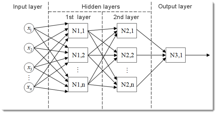
Fig. 2. The model of a multilayer neural network
This is what a multilayer neural network looks like. It comprises:
- The input layer which serves to distribute the data across the network and does not perform any calculations. The outputs of this layer transmit signals to the inputs of the next layer (hidden or output);
- The output layer which usually contains one neuron (or sometimes more than one) that generates the output of the entire neural network. This signal underlies the EA's future control logic;
- The hidden layers which are layers of standard neurons that transmit signals from the input layer to the output layer. Its input is the output of the previous layer, while its output serves as the input of the next layer.
This example has shown the neural network with two hidden layers. But there may be neural networks that have more hidden layers.
Input Data Normalization
Input data normalization is the process whereby all input data is normalized, i.e. reduced to the ranges [0,1] or [-1,1]. If normalization is not performed, the input data will have an additional effect on the neuron, leading to wrong decisions. In other words, how can you compare values that have different orders of magnitude?
The normalization formula in its standard form is as follows:

where:
 - value to be normalized;
 - х value range;
 - range to which the value of x will be reduced.
Let me explain it using an example:
Suppose, we have n input data from the range [0,10], then ![]() = 0 and
= 0 and ![]() = 10. We will reduce the data to the range [0,1], then
= 10. We will reduce the data to the range [0,1], then ![]() = 0 and
= 0 and ![]() = 1. Now, having plugged in the values into the formula, we can calculate normalized values for any x from n input data.
= 1. Now, having plugged in the values into the formula, we can calculate normalized values for any x from n input data.
This is what it looks like when implemented in MQL5:
double d1=0.0;
double d2=1.0;
double x_min=iMA_buf[ArrayMinimum(iMA_buf)];
double x_max=iMA_buf[ArrayMaximum(iMA_buf)];
for(int i=0;i<ArraySize(iMA_buf);i++)
  {
   inputs[i]=(((iMA_buf[i]-x_min)*(d2-d1))/(x_max-x_min))+d1;
  }
We first specify the output value upper and lower limits and then obtain the indicator minimum and maximum values (copying data from the indicator is left out but there can be, for instance, 10 last values). Lastly, we normalize every input element (indicator values on different bars) and store the results in an array for further use.
Activation Functions
The activation function is a function that calculates the output of a neuron. The input it receives represents the sum of all the products of the inputs and their respective weights (hereinafter "weighted sum"):

Fig. 3. The artificial neuron model with the activation function outlined
The activation function formula in its standard form is as follows:
![]()
where:
 is the activation function;
-
 is the weighted sum obtained at the first stage of calculating the output of a neuron;
  is a threshold value of the activation function. It is only used for the hard threshold function and is equal to zero in other functions.
Main types of activation functions are:
-
The unit step or hard threshold function.
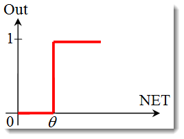
The function is described by the following formula:

If the weighted sum is less than the specified value, the activation function returns zero. If the weighted sum becomes greater, the activation function returns one. -
The sigmoid function.
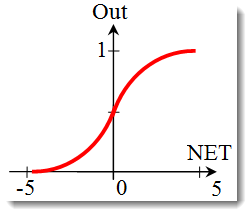
The formula that describes the sigmoid function is as follows:

It is often used in multilayer neural networks and other networks with continuous signals. The function smoothness and continuity are very positive properties. -
The hyperbolic tangent.
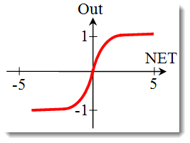
Formula:
 or
or 
It is also often used in networks with continuous signals. It is peculiar in that it can return negative values.
Changing the Activation Function Shape
In the previous section, we have dealt with the types of activation functions. Yet there is another important thing to be considered - the slope of a function (except for the hard threshold function). Let us take a closer look at the sigmoid function.
Looking at the function graph, one can easily see that the function is smooth over the range [-5,5]. Suppose we have a network consisting of a single neuron with 10 inputs and one output. Let us now try to calculate the upper and lower values of the variable ![]() . Every input will take a normalized value (as already mentioned in the Input Data Normalization), e.g. from the range [-1,1].
. Every input will take a normalized value (as already mentioned in the Input Data Normalization), e.g. from the range [-1,1].
We will use the negative input values since the function is differentiable even at a negative argument. Weights will also be selected from the same range. With all possible combinations of inputs and weights, we will get the extreme values ![]() in the range [-10,10] as:
in the range [-10,10] as:

In MQL5, the formula will look as follows:
for(int n=0; n<10; n++)
  {
   NET+=Xn*Wn;
  }
Now we need to plot the activation function in the range as identified. Let us take the sigmoid function as an example. The easiest way to do it is using Excel.
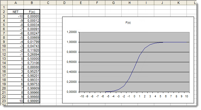
Fig. 4. The Excel graph of the sigmoid function
Here, we can clearly see that the argument values outside of the range [-5,5] have absolutely no effect on the results. This suggests that the range of values is incomplete. Let us try to fix this. We will add to the argument an additional coefficient d that will allow us to expand the range of values.
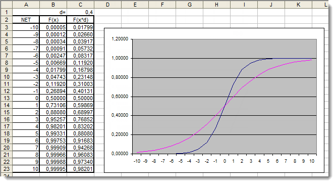
Fig. 5. The Excel graph of the sigmoid function with the additional coefficient applied
Let us once again have a look at the graphs. We have added an additional coefficient d=0.4 that changed the function shape. Comparison of the values in the table suggests that they are now more uniformly distributed. So the results can be expressed as follows:
for(int n=0; n<10; n++)
  {
   NET+=Xn*Wn;
  }
NET*=0.4;
Let us now review the hyperbolic tangent activation function. Skipping the theory covered in the review of the previous function, we get to practical application right away. The only difference here is that the output can lie in the range [-1,1]. The weighted sum can also take values from the range [-10,10].
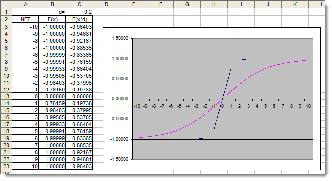
Fig. 6. The Excel graph of the hyperbolic tangent function with the additional coefficient applied
The graph shows that the shape of the function has been improved due to the use of the additional coefficient d=0.2. So the results can be expressed as follows:
for(int n=0;n<10;n++)
  {
   NET+=Xn*Wn;
  }
NET*=0.2;
In this manner, you can change and improve the shape of any activation function.
Application
Now let us move on to practical application. First, we will try to implement the calculation of the neuron's net input, followed by adding the activation function. Let us recall the formula for calculating the neuron's net input:

double NET;
double x[3];
double w[3];
int OnInit()
  {
   x[0]=0.1; // set the input value х1
   x[1]=0.8; // set the input value х2
   x[2]=0.5; // set the input value х3

   w[0]=0.5; // set the weight value w1
   w[1]=0.6; // set the weight value w2
   w[2]=0.3; // set the weight value w3

   for(int n=0;n<3;n++)
     {
      NET+=x[n]*w[n]; // add the weighted net input values together
     }
  }
Let us look into it:
- We have started with declaring a variable for storing the neuron's net input
 and two arrays: inputs
  and weights
  ;
; - Those variables have been declared at the very beginning, outside of all functions in order to give them a global scope (to be accessible from anywhere in the program);
- In the OnInit() initialization function (it can actually be any other function), we have filled the array of input and the array of weights;
- This was followed by the summing loop, n<3 since we only have three inputs and three respective weights;
- We then added weighted input values and stored them in the variable
 .
.
The first task has thus been completed - we have obtained the sum. Now it is the turn of the activation function. Below are the codes for calculating the activation functions reviewed in the Activation Functions section.
The unit step or hard threshold function
double Out;
if(NET>=x) Out=1;
else Out=0;
The sigmoid function
double Out = 1/(1+exp(-NET));
The hyperbolic tangent function
double Out = (exp(NET)-exp(-NET))/(exp(NET)+exp(-NET));
Putting It All Together
To make the implementation easier, we will take a network made up of a single neuron. It is certainly a bit of a stretch to call it a network but important is to understand the principle. After all, a multilayer neural network consists of the same neurons where the output of the previous layer of neurons serves as the input for the next layer.
We are going to use a slightly modified version of the Expert Advisor developed and introduced in the article "A Quick Start or a Short Guide for Beginners". Thus, we will for example replace the Moving Average trend indicator with the Relative Strength Index oscillator. Information on parameters of the indicator and their sequence can be found in the built-in Help.
//+------------------------------------------------------------------+
//|                                                neuro-example.mq5 |
//|                        Copyright 2012, MetaQuotes Software Corp. |
//|                                              http://www.mql5.com |
//+------------------------------------------------------------------+
#property copyright "Copyright 2012, MetaQuotes Software Corp."
#property link      "http://www.mql5.com"
#property version   "1.00"
//+------------------------------------------------------------------+
//| Expert initialization function                                   |
//+------------------------------------------------------------------+
#include <Trade\Trade.mqh>        //include the library for execution of trades
#include <Trade\PositionInfo.mqh> //include the library for obtaining information on positions

//--- weight values
input double w0=0.5;
input double w1=0.5;
input double w2=0.5;
input double w3=0.5;
input double w4=0.5;
input double w5=0.5;
input double w6=0.5;
input double w7=0.5;
input double w8=0.5;
input double w9=0.5;

int               iRSI_handle;  // variable for storing the indicator handle
double            iRSI_buf[];   // dynamic array for storing indicator values

double            inputs[10];   // array for storing inputs
double            weight[10];   // array for storing weights

double            out;          // variable for storing the output of the neuron

string            my_symbol;    // variable for storing the symbol
ENUM_TIMEFRAMES   my_timeframe; // variable for storing the time frame
double            lot_size;     // variable for storing the minimum lot size of the transaction to be performed

CTrade            m_Trade;      // entity for execution of trades
CPositionInfo     m_Position;   // entity for obtaining information on positions
//+------------------------------------------------------------------+
//|                                                                  |
//+------------------------------------------------------------------+
int OnInit()
  {
//--- save the current chart symbol for further operation of the EA on this very symbol
   my_symbol=Symbol();
//--- save the current time frame of the chart for further operation of the EA on this very time frame
   my_timeframe=PERIOD_CURRENT;
//--- save the minimum lot of the transaction to be performed
   lot_size=SymbolInfoDouble(my_symbol,SYMBOL_VOLUME_MIN);
//--- apply the indicator and get its handle
   iRSI_handle=iRSI(my_symbol,my_timeframe,14,PRICE_CLOSE);
//--- check the availability of the indicator handle
   if(iRSI_handle==INVALID_HANDLE)
     {
      //--- no handle obtained, print the error message into the log file, complete handling the error
      Print("Failed to get the indicator handle");
      return(-1);
     }
//--- add the indicator to the price chart
   ChartIndicatorAdd(ChartID(),0,iRSI_handle);
//--- set the iRSI_buf array indexing as time series
   ArraySetAsSeries(iRSI_buf,true);
//--- place weights into the array
   weight[0]=w0;
   weight[1]=w1;
   weight[2]=w2;
   weight[3]=w3;
   weight[4]=w4;
   weight[5]=w5;
   weight[6]=w6;
   weight[7]=w7;
   weight[8]=w8;
   weight[9]=w9;
//--- return 0, initialization complete
   return(0);
  }
//+------------------------------------------------------------------+
//| Expert deinitialization function                                 |
//+------------------------------------------------------------------+
void OnDeinit(const int reason)
  {
//--- delete the indicator handle and deallocate the memory space it occupies
   IndicatorRelease(iRSI_handle);
//--- free the iRSI_buf dynamic array of data
   ArrayFree(iRSI_buf);
  }
//+------------------------------------------------------------------+
//| Expert tick function                                             |
//+------------------------------------------------------------------+
void OnTick()
  {
//--- variable for storing the results of working with the indicator buffer
   int err1=0;
//--- copy data from the indicator array to the iRSI_buf dynamic array for further work with them
   err1=CopyBuffer(iRSI_handle,0,1,10,iRSI_buf);
//--- in case of errors, print the relevant error message into the log file and exit the function
   if(err1<0)
     {
      Print("Failed to copy data from the indicator buffer");
      return;
     }
//---
   double d1=0.0;                                 //lower limit of the normalization range
   double d2=1.0;                                 //upper limit of the normalization range
   double x_min=iRSI_buf[ArrayMinimum(iRSI_buf)]; //minimum value over the range
   double x_max=iRSI_buf[ArrayMaximum(iRSI_buf)]; //maximum value over the range

//--- In the loop, fill in the array of inputs with the pre-normalized indicator values
   for(int i=0;i<ArraySize(inputs);i++)
     {
      inputs[i]=(((iRSI_buf[i]-x_min)*(d2-d1))/(x_max-x_min))+d1;
     }
//--- store the neuron calculation result in the out variable
   out=CalculateNeuron(inputs,weight);
//--- if the output value of the neuron is less than 0.5
   if(out<0.5)
     {
      //--- if the position for this symbol already exists
      if(m_Position.Select(my_symbol))
        {
         //--- and this is a Sell position, then close it
         if(m_Position.PositionType()==POSITION_TYPE_SELL) m_Trade.PositionClose(my_symbol);
         //--- or else, if this is a Buy position, then exit
         if(m_Position.PositionType()==POSITION_TYPE_BUY) return;
        }
      //--- if we got here, it means there is no position; then we open it
      m_Trade.Buy(lot_size,my_symbol);
     }
//--- if the output value of the neuron is equal to or greater than 0.5
   if(out>=0.5)
     {
      //--- if the position for this symbol already exists
      if(m_Position.Select(my_symbol))
        {
         //--- and this is a Buy position, then close it
         if(m_Position.PositionType()==POSITION_TYPE_BUY) m_Trade.PositionClose(my_symbol);
         //--- or else, if this is a Sell position, then exit
         if(m_Position.PositionType()==POSITION_TYPE_SELL) return;
        }
      //--- if we got here, it means there is no position; then we open it
      m_Trade.Sell(lot_size,my_symbol);
     }
  }
//+------------------------------------------------------------------+
//|   Neuron calculation function                                    |
//+------------------------------------------------------------------+
double CalculateNeuron(double &x[],double &w[])
  {
//--- variable for storing the weighted sum of inputs
   double NET=0.0;
//--- Using a loop we obtain the weighted sum of inputs based on the number of inputs
   for(int n=0;n<ArraySize(x);n++)
     {
      NET+=x[n]*w[n];
     }
//--- multiply the weighted sum of inputs by the additional coefficient
   NET*=0.4;
//--- send the weighted sum of inputs to the activation function and return its value
   return(ActivateNeuron(NET));
  }
//+------------------------------------------------------------------+
//|   Activation function                                            |
//+------------------------------------------------------------------+
double ActivateNeuron(double x)
  {
//--- variable for storing the activation function results
   double Out;
//--- sigmoid
   Out=1/(1+exp(-x));
//--- return the activation function value
   return(Out);
  }
//+------------------------------------------------------------------+
The first thing we need to do is to train our network. Let us optimize the weights.
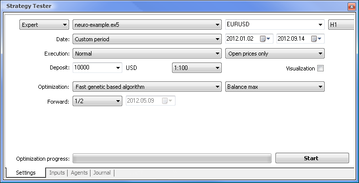
Fig. 7. Strategy tester with the required parameters set
We will run the optimization using the following parameters:
- Date - e.g. from the beginning of the year The longer the period, the less the occurrence of curve fitting and the better the result.
- Execution - normal, Opening prices only. There is no point in testing in Every tick mode since our Expert Advisor only takes 10 last values of the indicator, except for the current value.
- Optimization can be set to run using the slow complete algorithm. Genetic optimization will however give faster results which comes in particularly handy when assessing an algorithm. If the result is satisfying, you can also try using the slow complete algorithm for more accurate results.
- Forward of 1/2 and more allows you to assess how long your EA can generate the obtained results until the next optimization.
- Time frame and Currency pair can be set as you deem fit.
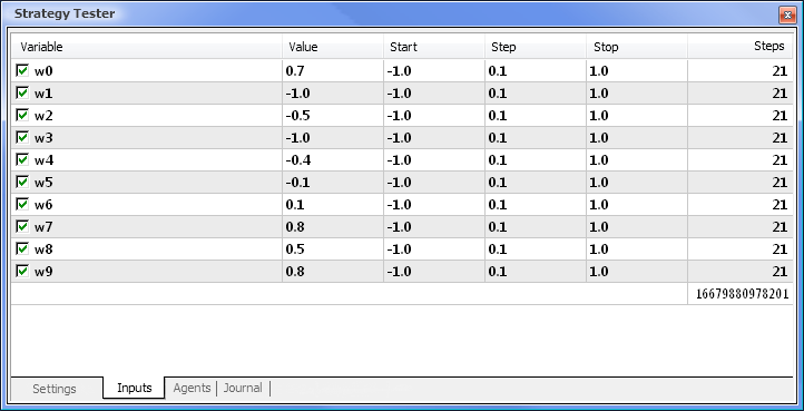
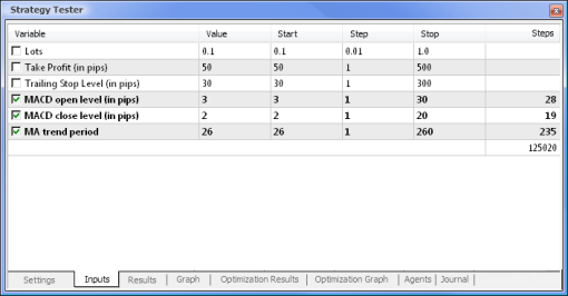
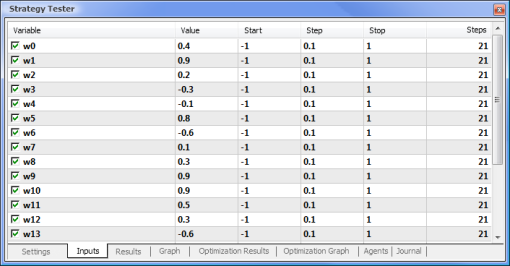
Fig. 8. Setting the parameters and their respective ranges to be optimized
The optimization will be run with respect to all weights and their ranges. Start the optimization by going back to the Settings tab and clicking on the Start button.
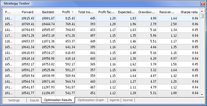
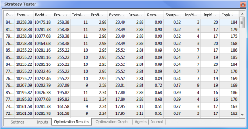
Fig. 9. Data obtained following the optimization
After the optimization is complete, we select the pass with the maximum profit value (to sort by one of the parameters, click on the relevant column heading) in the Optimization Results tab. You can then assess other parameters and select the desired pass, if necessary.
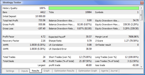
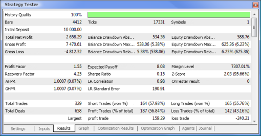
A double click on the required pass initiates testing the results of which are shown in the Results and Graph tabs.
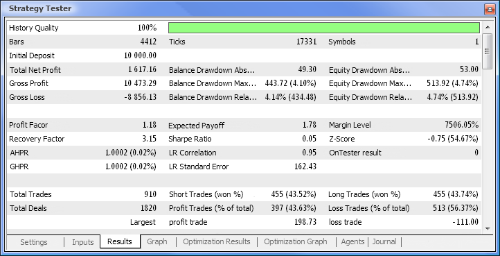
Fig. 10. Test report
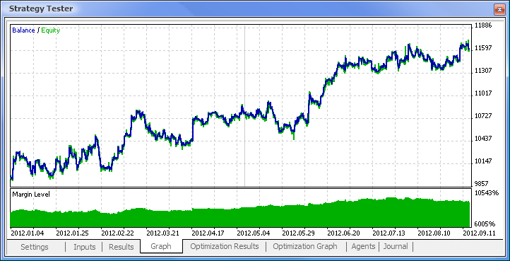
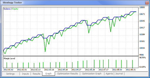
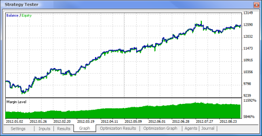
Fig. 11. Balance chart
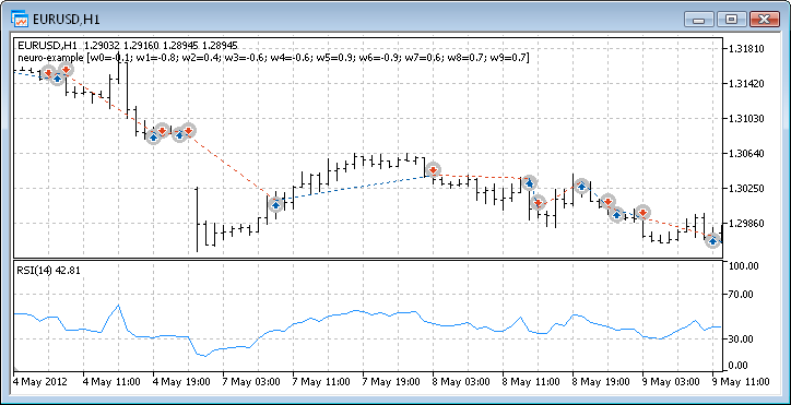
Fig. 12. Trading performance of the Expert Advisor
So we have finally got the results and for a start they are not bad at all. Bear in mind that we only had one neuron. The example provided is clearly primitive but we must admit that even it alone can earn profit.
Advantages of Neural Networks
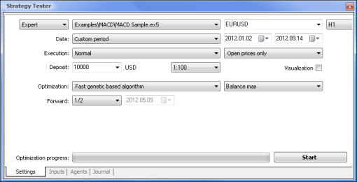
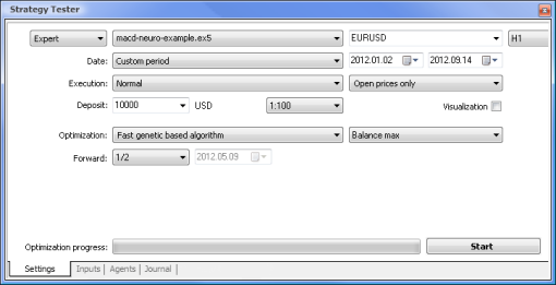
Let us now try to compare an EA based on the standard logic with a neural network driven EA. We will compare the optimization and testing results of the MACD Sample Expert Advisor that comes together with the terminal with those of the neural network driven EA based on MACD.
Take Profit and Trailing Stop values will not be involved in the optimization as they are missing from the neural network driven EA. Both Expert Advisors that we are going to test are based on MACD with the following parameters:
- Period of the fast moving average: 12;
- Period of the slow moving average: 26;
- Period of averaging of the difference: 9;
- Price type: closing price.
You can also set the required currency pair and time frame but in our case we will leave them unchanged - EURUSD, H1, respectively. The testing period in both cases is the same: from the beginning of the year using opening prices.
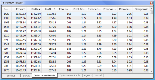
| MACD Sample | macd-neuro-examle |
|---|---|
 |
 |
 |
 |
 |
 |
 |
 |
 |
 |
Let us now compare the key parameters of the tested Expert Advisors:
| Parameter | MACD Sample | macd-neuro-examle |
|---|---|---|
| Total Net Profit | 733,56 | 2 658,29 |
| Balance Drawdown Absolute | 0,00 | 534,36 |
| Equity Drawdown Maximal | 339,50 (3,29%) | 625,36 (6,23%) |
| Profit Factor | 4,72 | 1,55 |
| Recovery Factor | 2,16 | 4,25 |
| Expected Payoff | 30,57 | 8,08 |
| Sharpe Ratio | 0,79 | 0,15 |
| Total Trades | 24 | 329 |
| Total Deals | 48 | 658 |
| Profit Trades (% of total) | 21 (87,50%) | 187 (56,84%) |
| Average Profit Trade | 44,33 | 39,95 |
| Average Consecutive Wins | 5 | 2 |
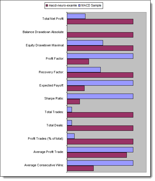
Fig. 13. Comparison of the key parameters
Conclusion
This article has covered the main points you need to know when designing EAs using neural networks. It has shown us the structure of a neuron and neural network architecture, outlined the activation functions and the methods for changing the activation function shape, as well as the process of optimization and input data normalization. Furthermore, we have compared an EA based on the standard logic with a neural network driven EA.
Translated from Russian by MetaQuotes Ltd.
Original article: https://www.mql5.com/ru/articles/497
Warning: All rights to these materials are reserved by MetaQuotes Ltd. Copying or reprinting of these materials in whole or in part is prohibited.
This article was written by a user of the site and reflects their personal views. MetaQuotes Ltd is not responsible for the accuracy of the information presented, nor for any consequences resulting from the use of the solutions, strategies or recommendations described.
 Order Strategies. Multi-Purpose Expert Advisor
 MetaTrader 5 on Linux
 General information on Trading Signals for MetaTrader 4 and MetaTrader 5
- Free trading apps
- Over 8,000 signals for copying
- Economic news for exploring financial markets
You agree to website policy and terms of use
only opens 1 trade in backtest
An important question:
The RSI N past values is set to 14(N=14).
The number of inputs is 10 (past values).
Is there a problem? Seems that the ML results might be unstable?
Please answer....
Thanks
An important question:
The RSI N past values is set to 14(N=14).
The number of inputs is 10 (past values).
Is there a problem? Seems that the ML results might be unstable?
Please answer....
Thanks
14 is the period to calculate RSI indicator. Input is 10 values from the RSI buffer.