Self Optimizing Expert Advisors in MQL5 (Part 11): A Gentle Introduction to the Fundamentals of Linear Algebra

In our opening discussion on matrix factorization, we explored the many benefits of using the linear algebra commands available in the MQL5 API. That initial discussion assumed that the reader had some prerequisite knowledge—namely, a foundational understanding of time series modeling and statistical analysis. However, in retrospect, it is clear that this assumption may not hold true for all readers.

If this is your first time encountering such topics, the introductory article may not have been as helpful as intended. The content advanced quickly, with many concepts introduced in rapid succession. Therefore, in this article, I aim to shift focus toward readers with no prior experience whatsoever in the mathematical techniques being introduced.

I will present these techniques from a perspective that assumes no background knowledge, ensuring that all readers can follow along and appreciate the value of the matrix and vector API. The matrix and vector API provided by MQL5 is indeed powerful, but it is not sufficient on its own. It does not operate independently. Only by understanding the principles of linear algebra can we make intelligent and effective use of this API.

This article will serve as a bridge for readers without formal mathematical instruction. We will adopt a comparative style of teaching: I will begin by illustrating code that might be written by an MQL5 developer without a background in linear algebra, and then compare that to code written by someone who does understand the underlying mathematical principles. This side-by-side approach will allow the benefits of linear algebra to stand out clearly and intuitively.

All theoretical concepts introduced will be directly tied to practical trading applications, which we will demonstrate right here in the MetaTrader 5 terminal. Using real market data, we will apply the mathematical theory in a hands-on manner, showcasing the versatility and practical value of these linear algebra commands.

Today, we will build a statistical model that predicts multiple targets simultaneously. Typically, linear regression models are used to project a single target—for example, the future change in price. However, in this case, we aim to predict four different targets:

• The future moving average of the close
• The future moving average of the high
  
• The future moving average of the low
  
• The future value of price

We will incorporate these predictions into our trading strategy to define both entry and exit rules, as well as filters for closing positions. The Matrix and Vector MQL5 API offers us powerful tools for building modern machine learning applications. But to realize the potential of the API, you must appreciate the basic linear algebra rules that stand behind the appropriate usage of these dedicated methods.

Linear Algebra can often be an abstract mathematical study. However, I wish to bring the subject to life for you so you can clearly see the benefits of what we are about to cover, and then we will discuss the mathematical towards the middle of the discussion. Finally, after the motivation of our discussion is clear,  and all the requisite mathematical notation has been explained, we will demonstrate one example of how to employ linear algebra to build numerically driven trading algorithms capable of forecasting multiple targets simultaneously. 

Maintainable Codebase

Most of the time, when dealing with market prices—such as collections of the open, high, low, and close prices—it is helpful to store this data in matrix form. In MQL5, matrices are indexed by row first, followed by column. Therefore, we begin by defining a new matrix A, which is 3 by 5 and initialized with zeros. This means that matrix A will have three rows and five columns, and all entries will initially be set to zero. We then display matrix A in its current state, which, as shown in Figure 1, is indeed filled with zeros.

//--- Let's first create an empty matrix
matrix A=matrix::Zeros(3,5);

//--- Peek at the matrix
Print("Original A matrix");
Print(A);

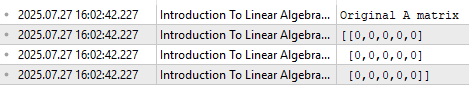
Figure 1: Visualizing our blank matrix A

Next, we label each of the rows: row one will be filled with constant values of one, row two with values of two, and row three with values of three.

As the reader can observe, the notation used to access elements inside a matrix in MQL5 always begins with the row index, followed by the column index inside square brackets, placed next to the identifier associated with the matrix. We can inspect matrix A once again to confirm it has been filled correctly—Figure 2 assures us that it has.

//--- The notation A[R,C] describes the Row and Column we want to manipulate
//--- We will set all the values in Row 1 to be 1
A[0,0] = 1;
A[0,1] = 1;
A[0,2] = 1;
A[0,3] = 1;
A[0,4] = 1;

//--- We will set all the values in Row 2 to be 2
A[1,0] = 2;
A[1,1] = 2;
A[1,2] = 2;
A[1,3] = 2;
A[1,4] = 2;

//--- We will set all the values in Row 3 to be 3
A[2,0] = 3;
A[2,1] = 3;
A[2,2] = 3;
A[2,3] = 3;
A[2,4] = 3;

Print("Current A matrix");
Print(A);

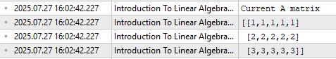
Figure 2: Labelling the rows in our matrix A for our exercise

Now, let us manipulate the values inside our matrix. Suppose we want to multiply all the values in the second row of matrix A by five. A naive implementation might involve creating a for loop to iterate over each entry in row two, multiply each by five, and store the result. As we can see, this approach achieves the desired outcome and would pass any functional test.

However, can the reader think of reasons why we might want to avoid using a for loop for this task?

//--- Let's multiply all the values of Row 2 by 5 and leave all the other rows the same.

//--- Bad performing code
//--- Copy matrix A
matrix example_1;
example_1.Assign(A);

//--- Loop over matrix A and multiply each element by 5 and then replace the original elements
for(int i =0;i<5;i++)
{
   example_1[1,i] = example_1[1,i] * 5;
}

//--- Done
Print("Example 1: ");
Print(example_1);

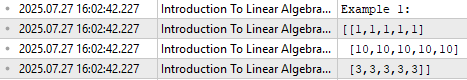
Figure 3: Manipulating matrix A using a for loop may become too slow as A grows large

Let us consider a slightly improved approach. Instead of looping, we could select the second row of the matrix as a row vector, multiply it by five, and then assign the result back to its original position. This produces the same effect and is more elegant. Still, I ask the reader again: can you think of why even this might not be the best possible approach?

//--- Slightly better code
//--- Copy the row, multiply it and then put it back
matrix example_2;
vector copy_vector;

example_2.Assign(A);

copy_vector = example_2.Row(1);

example_2.Row(copy_vector*5,1);

Print("Example 2");
Print(example_2);

Figure 4: Manipulating matrix A using vector methods is better than a traditional for loop, but not optimal

Finally, I will demonstrate what is considered a suitable approach in this context: we begin by creating a scaling vector and then use matrix multiplication to apply this vector to matrix A. As shown, all three code snippets produce the same result. However, the reader should notice several important differences.

The third approach requires the fewest lines of code. This demonstrates a key advantage of using linear algebra for our daily trading tasks: it allows us to write more concise, maintainable code. For most developers, I believe this alone should be a compelling reason to invest time in learning linear algebra. However, there are many more benefits I will demonstrate as we proceed. This is simply a good place to start.

//--- Reliable code
matrix example_3,scaler;
vector scale = {1,5,1};

scaler.Diag(scale);
example_3 = scaler.MatMul(A);

//--- Done 
Print("Example 3");
Print(example_3);

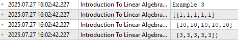
Figure 5: Using appropriate matrix and vector dedicated methods when they exist is always best

Now let us extend the example. Initially, we multiplied only the second row by five. Let us now multiply the first row by two, the last row by ten, and leave the middle row unchanged. At this point, the reader may start to see the issues with using the for loop. As the number of operations on matrix A increases, so too does the length of our loop—and thus the number of lines we must write. Moreover, if matrix A is sufficiently large, iterating over each value one by one—as suggested by the loop—can significantly slow down execution, especially during backtesting. 

//--- Now, multiply the first and last rows by 2 and 10, but leave the middle row as it is.

//--- Loops can slow us down during backtests, especially if they must be repeated often.
for(int i =0;i<5;i++)
{
   example_1[0,i] = example_1[0,i] * 2;
   example_1[2,i] = example_1[2,i] * 10;
}

//--- Done
Print("Example 1");
Print(example_1);

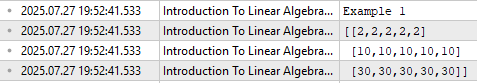
Figure 6: We have to write more lines of code in our for loop, just to obtain the same effect

Similarly, using the method of selecting and reassigning individual rows grows increasingly complex as the number of operations increases. Although this method is superior to a basic for loop, it still leads to bloated code, increasing the likelihood of errors.

//--- The difference between example 2 and 3 starts to show
//--- Copy the row, multiply it and then put it back
vector copy_vector_2;

copy_vector = example_2.Row(0);
copy_vector_2 = example_2.Row(2);

example_2.Row(copy_vector*2,0);
example_2.Row(copy_vector_2*10,2);

//--- Done
Print("Example 2");
Print(example_2);

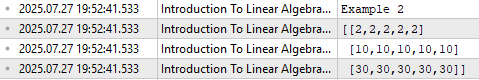
Figure 7: Chaining together general matrix and vector methods can still get the job done, but we can do better

We can still do better by relying on matrix multiplication. With this approach, the only thing that changes are the scaling values. The rest of the code remains essentially the same, regardless of the number of rows involved. All three methods produce the same output—but after seeing them side-by-side, I ask the reader: which approach seems most appropriate when working with large volumes of historical market data?

//--- Reliable code
vector scale_2 = {2,1,10};
scaler.Diag(scale_2);
example_3 = scaler.MatMul(example_3);

//--- Done
Print("Example 3");
Print(example_3);

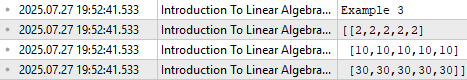
Figure 8: We can get the same output with fewer lines of code, by programming more concisely

Time Required To Backtest

With traditional for loops, we may not be able to process all data points efficiently, especially during time-sensitive operations like backtesting. This brings us to a second key point: not only is our codebase easier to maintain when using matrix and vector APIs appropriately, but the execution time of our trading strategies becomes more efficient as well.

At the end of the day, most readers are likely interested in building powerful AI models for trading—models capable of making informed decisions. But for your AI model to make such decisions, it needs access to large volumes of data. And before we feed that data into the model, we must perform certain preprocessing steps and manipulations.

If we perform these operations inefficiently, the number of lines required to build the application grows rapidly—especially if we rely on for loops. As code size increases, the time required for backtesting also increases.

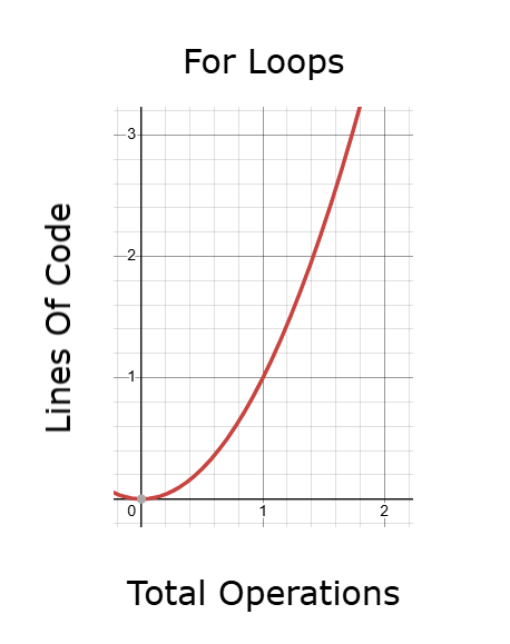
Figure 9: For loops may produce code that takes too long to run during back tests

A better alternative is to use chained vector and matrix operations. This method is much faster than traditional looping, but even it can become cumbersome if it involves repeatedly copying, modifying, and reassigning rows. If the number of such operations grows, so does the time needed to run the code, once again affecting backtest performance and model optimization.

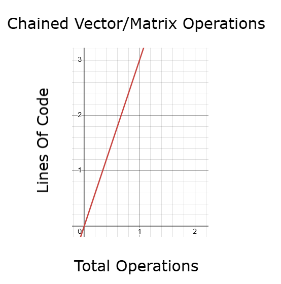
Figure 10: Chaining matrix and vector API's will be faster than a for loop, but we may be able to do better

On the other hand, by using the appropriate vector and matrix operations grounded in linear algebra, we can control execution time and keep code length and back test time constant—even as data size increases. This is a highly desirable quality in any application. It means we can perform more operations without always writing proportionally more code and without increasing execution time—allowing us to iterate and optimize machine learning models more effectively. I believe that most readers will be amazed at how much progress can be made simply by understanding a few fundamental concepts from linear algebra. We do not need advanced theory to begin seeing meaningful improvements in our applications.

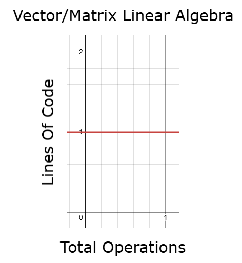
Figure 11: Employing linear algebra can help us achieve constant run-time from our applications

Precision

I would also like to emphasize an important issue that, in my view, is often overlooked in technical discussions: precision. I believe this subject does not receive the attention and scrutiny it truly deserves. Precision is one of the key components in building a reliable trading strategy. The results obtained from backtesting must be accurate, and the internal calculations and decisions made by the application are expected to be precise and trustworthy.

Consider the following scenario: in the example code snippet, we perform a basic floating-point subtraction—0.3 - 0.1. The computer reports the result as 0.199999... instead of the expected 0.2. This is a well-known issue in computer science related to floating-point arithmetic, and it is not unique to MQL5. 

The point I want to stress is this: imagine performing such a subtraction operation inside a loop. Now, imagine looping through a matrix like A, which may have over a million rows, performing this operation on each one. It becomes easy to see how these small errors in precision can accumulate and compound, eventually introducing significant numerical instability into your results.

Performing arithmetic carelessly—such as direct subtractions like this on large matrices—is inefficient and will not produce results that are precise or numerically stable.

Furthermore, when we consider algorithms like those shown in earlier examples—where values are repeatedly copied from one place to another, new objects are created, data is reassigned, and memory is constantly being allocated and deallocated—the issue becomes even more pressing. Computers have limited memory. When we perform matrix operations inefficiently, constantly generating and destroying objects, we increase memory pressure unnecessarily. Trying to manage memory in such a haphazard way has material consequences that we often overlook.

Moreover, there are known algorithms—many of which are already implemented in MQL5’s matrix and vector API, as well as in supporting libraries we will cover—that are designed with these exact issues in mind. These implementations are optimized to minimize floating-point error and maximize numerical stability. In contrast, when developers opt for less efficient methods—such as manual for loops for data manipulation—they unknowingly increase the likelihood of encountering these problems.

//--- Why should you care?
//--- Let's start with an often overlooked need, precision!
Print("Our computers have limited memory to store numbers with precision");
Print("What is 0.3 - 0.1");
Print(0.3-0.1);
Print("You and I know the correct answer is 0.2");

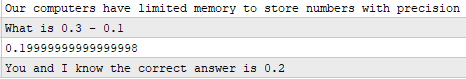
Figure 12: Using the appropriate matrix/vector linear algebra can help us minimize such errors

How Can We Use Linear Algebra As Traders?

Now that the reader has developed an appreciation for the advantages of learning linear algebra, it’s time to consider some of the foundational rules that govern how we make decisions using it. Understanding these core rules is a valuable skill.

Beginner's Note: My goal here is not to get you to memorize formulas. Rather, it is to help you understand the principles deeply enough that they become intuitive—so you will remember them naturally, not through rote learning.

To begin understanding linear algebra, we first need a solid grasp of basic algebra. Algebra is essentially the mathematics of unknown quantities. Let’s start with a simple example, illustrated in Figure 13: This equation is saying: some unknown value , when multiplied by 2, gives 4. To solve for x, we divide both sides by 2. If we want to test our solution, simply replace x with the value 2 in the original equation and then check if 2 multiplied by 2 is indeed 4. While this may feel basic, it sets the stage for more advanced concepts.

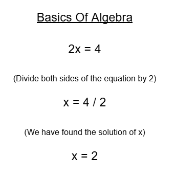
Figure 13: Visualizing a simple problem in algebra where the value of x is 2

Now, let’s consider a slight variation: what if the equation were A multiplied by 2, gives 4. We would divide both sides by A and give the solution as x is equal to 4 divided by A. Because we are not told what A is equal to, we have finished solving the question.

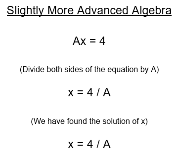
Figure 14: Considering a slightly more complicated version of the problem depicted in Figure 13

Now, what happens if A isn’t just a number—but a matrix? This is where we transition from the algebra taught in high school to linear algebra. Here, is A matrix. We might be tempted to divide both sides by A, as we did earlier. But in linear algebra, division by a matrix is not defined. Instead, we use the inverse of a matrix. If the matrix has an inverse, we solve the equation by multiplying both sides by the inverse of A.

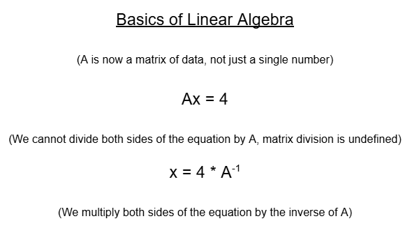
Figure 15: Linear algebra relies on the same logic we used for our simple examples, but we just modify a few rules

What does this mean in the context of market data? Suppose matrix A represents current market data—such as price levels. The vector y represents the future price you’re trying to predict. You want to find the coefficient vector such that “When I multiply my current data by the coefficient vector , I should get the future price levels.”

But here’s the problem: not every matrix has an inverse. In fact, inverting a matrix that is not invertible can crash your trading algorithm or return unreliable results. For this reason, we do not "blindly" invert any matrix that we come across. Instead, it is often safer and more stable to work with smaller submatrices of —portions of the data that we can reliably invert or process using other numerically stable techniques, like matrix factorizations (e.g., QR, SVD, or pseudo-inverses).

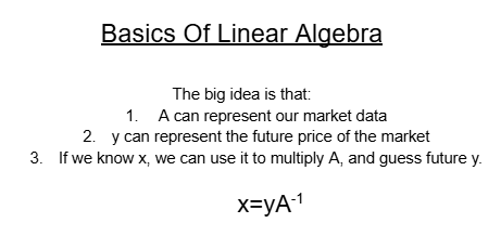
Figure 16: Generalizing the solution to any linear system of equations

Using Linear Algebra To Improve Our Trading

Now that we have developed a level of familiarity with the basic rule of solving linear systems of equations using linear algebra, we are ready to begin applying what we have learned about solving for the coefficient vector x. For this particular example, I want to show you that the formula we discussed can solve for multiple targets in y just as easily as it can solve for a single target. So, let us begin by defining our system constants. Today, we need to specify how many inputs our model will take. This particular model will take eight inputs.

//+------------------------------------------------------------------+
//|                                            Linear Regression.mq5 |
//|                                               Gamuchirai Ndawana |
//|                    https://www.mql5.com/en/users/gamuchiraindawa |
//+------------------------------------------------------------------+
#property copyright "Gamuchirai Ndawana"
#property link      "https://www.mql5.com/en/users/gamuchiraindawa"
#property version   "1.00"

//+------------------------------------------------------------------+
//| System constants                                                 |
//+------------------------------------------------------------------+
#define TOTAL_INPUTS 8

Afterward, we must define important system parameters. For example, the number of historical bars to fetch, how far ahead into the future we want to forecast, the time frames we are using, and other related settings. All of these details will be stored in the system parameters.

//+------------------------------------------------------------------+
//| System parameters                                                |
//+------------------------------------------------------------------+
int bars = 90;                                        //Number of historical bars to fetch
int horizon = 1;                                      //How far into the future should we forecast
int MA_PERIOD = 2;                                    //Moving average period
ENUM_TIMEFRAMES TIME_FRAME = PERIOD_D1;               //User Time Frame
ENUM_TIMEFRAMES RISK_TIME_FRAME = PERIOD_D1;          //Time Frame for our ATR stop loss
double sl_size = 2;                                   //ATR Stop loss size

Dependencies in any application are important because they reduce the total amount of code that has to be rewritten from one project to the next. Therefore, we will load several key dependencies—such as the Trade Impedance dependency, which comes preinstalled with every version of MetaTrader 5. The remaining two dependencies were custom-written for our trading activities.

//+------------------------------------------------------------------+
//| Dependencies                                                     |
//+------------------------------------------------------------------+
#include <Trade\Trade.mqh>
#include <VolatilityDoctor\Time\Time.mqh>
#include <VolatilityDoctor\Trade\TradeInfo.mqh>

Our system will also define important global variables that will be used across different contexts within the application. For example, we will have global variables to store the current indicator readings. Others will store values used by the dependencies, and still others will hold the coefficients we've learned from the data. These include values like the ATR reading and many other moving parts of our system.

//+------------------------------------------------------------------+
//| Global Variables                                                 |
//+------------------------------------------------------------------+
int        ma_close_handler,ma_high_handler,ma_low_handler;
double     ma_close[],ma_high[],ma_low[];
Time       *Timer;
TradeInfo  *TradeInformation;
vector     bias,temp,temp_2,temp_3,temp_4,temp_5,Z1,Z2;
matrix     X,y,prediction,b;
int        time;
CTrade Trade;
int state;
int atr_handler;
double atr[];

Upon initialization, the system will create new objects for the custom dependencies we loaded. The timer is responsible for tracking the formation of new candles. The trade formation module returns important information such as the minimum trading volume, the ask price, and the bid. We will also create handlers for tracking our moving averages, as well as initialize our matrices and vectors with placeholder values of one just to get us started.

//+------------------------------------------------------------------+
//| Expert initialization function                                   |
//+------------------------------------------------------------------+
int OnInit()
  {
//---
   Timer                   = new Time(Symbol(),TIME_FRAME);
   TradeInformation        = new TradeInfo(Symbol(),TIME_FRAME);
   ma_close_handler        = iMA(Symbol(),TIME_FRAME,MA_PERIOD,0,MODE_SMA,PRICE_CLOSE);
   ma_high_handler        = iMA(Symbol(),TIME_FRAME,MA_PERIOD,0,MODE_SMA,PRICE_HIGH);
   ma_low_handler        = iMA(Symbol(),TIME_FRAME,MA_PERIOD,0,MODE_SMA,PRICE_LOW);

   bias = vector::Ones(TOTAL_INPUTS);
   Z1 = vector::Ones(TOTAL_INPUTS);
   Z2 = vector::Ones(TOTAL_INPUTS);
   X = matrix::Ones(TOTAL_INPUTS,bars);
   y = matrix::Ones(1,bars);
   time = 0;
   state = 0;
   atr_handler = iATR(Symbol(),RISK_TIME_FRAME,14);
//---
   return(INIT_SUCCEEDED);
  }

When our application is no longer in use, we will release any objects tied to memory resources. This is good practice in MQL5 and we will always follow it.

//+------------------------------------------------------------------+
//| Expert deinitialization function                                 |
//+------------------------------------------------------------------+
void OnDeinit(const int reason)
  {
//---
   IndicatorRelease(atr_handler);
   IndicatorRelease(ma_close_handler);
   IndicatorRelease(ma_high_handler);
   IndicatorRelease(ma_low_handler);
  }

Whenever updated prices are received in the OnTick handler, we first check if a new candle has fully formed. If it has, then we copy all the indicator readings into their associated arrays and prepare the model to make a market prediction. Once that's done, we track the current close price and calculate our stop loss—both for selling and buying positions.

From there, we display the predicted price levels that our model expects. Recall that we are forecasting the close moving average, the high moving average, the low moving average, and the price itself. If no positions are currently open, we first reset the relevant state variables. Then, we check the relationship between the expected close price and the expected close moving average in the future.

Generally, we want to see that our algorithm expects the moving average of the close to be above the current close price. This suggests that prices are currently undervalued—since they are trading below what the model considers fair value.

For additional confirmation, we also want to ensure that our stop loss is unlikely to get hit—both for buy and sell positions. In buy conditions, we verify that the low moving average is not expected to drop below the buy stop loss. In sell conditions, we check that the high moving average is not expected to rise above the sell stop loss. If either condition is violated, we avoid entering a position.

Additionally, we compare each individual moving average with its complementary pair. When buying, we expect the future value of the low moving average to be greater than its current value. When selling, we expect the future value of the low moving average to be lower than its current value. Similarly, when buying, we want the future high moving average to exceed its current value.

When it's time to close a position, we first check if prices are expected to move against us. If we anticipate that any moving average might exceed the stop loss, we immediately exit the trade. Otherwise, we allow the stop loss to continue trailing into more profitable territory.

//+------------------------------------------------------------------+
//| Expert tick function                                             |
//+------------------------------------------------------------------+
void OnTick()
  {
//---
   if(Timer.NewCandle())
     {
      CopyBuffer(atr_handler,0,0,1,atr);
      CopyBuffer(ma_close_handler,0,0,1,ma_close);
      CopyBuffer(ma_low_handler,0,0,1,ma_low);
      CopyBuffer(ma_high_handler,0,0,1,ma_high);

      setup();

      double c =  iClose(Symbol(),TIME_FRAME,0);
      double buy_sl = (TradeInformation.GetBid() - (sl_size * atr[0]));
      double sell_sl = (TradeInformation.GetAsk() + (sl_size * atr[0]));


      Comment("Forecasted MA: ",prediction[0,0],"\nForecasted MA High: ",prediction[1,0],"\nForecasted MA Low: ",prediction[2,0],"\nForecasted Price: ",prediction[3,0]);

      if(PositionsTotal() == 0)
        {
         state = 0;
         if((prediction[0,0] > c) && (prediction[2,0] > buy_sl) && (prediction[3,0] > c) && (prediction[2,0] > ma_low[0]) && (prediction[1,0] > ma_high[0]))
           {
            Trade.Buy(TradeInformation.MinVolume(),Symbol(),TradeInformation.GetAsk(),buy_sl,0);
            state = 1;
           }
         if((prediction[0,0] < c) && (prediction[1,0] < sell_sl) && (prediction[3,0] < c) && (prediction[2,0] < ma_low[0]) && (prediction[1,0] < ma_high[0]))
           {
            Trade.Sell(TradeInformation.MinVolume(),Symbol(),TradeInformation.GetBid(),sell_sl,0);
            state = -1;
           }
        }

      if(PositionsTotal() > 0)
        {
         double current_sl = PositionGetDouble(POSITION_SL);
        
         if(((state == -1) && (prediction[0,0] > c) && (prediction[1,0] > current_sl)) || ((state == 1)&&(prediction[0,0] < c)&& (prediction[2,0] < current_sl)))
            Trade.PositionClose(Symbol());
         if(PositionSelect(Symbol()))
           {
            

            if((state == 1) && ((ma_close[0] - (2 * atr[0]))>current_sl))
              {
               Trade.PositionModify(Symbol(),(ma_close[0] - (2 * atr[0])),0);
              }

            else
               if((state == -1) && ((ma_close[0] + (1 * atr[0]))<current_sl))
                 {
                  Trade.PositionModify(Symbol(),(ma_close[0] + (2 * atr[0])),0);
                 }
           }
        }
     }
  }

Next, we must discuss some of the individual functions prepared for the tasks above. The first function is prepare_data(). This function serves a single core purpose: it copies all the price levels we need into the input data matrix x. It fetches the open price, calculates the mean and standard deviation of the open price, and normalizes the data by subtracting the mean and dividing by the standard deviation. This process is repeated for all inputs. All the moving average handler values are also copied and stored into the target array y.

//+------------------------------------------------------------------+
//| Prepare the training data for our model                          |
//+------------------------------------------------------------------+
void prepare_data(void)
  {
//--- Reshape the matrix
   X = matrix::Ones(TOTAL_INPUTS,bars);

//--- Store the Z-scores
   temp.CopyRates(Symbol(),TIME_FRAME,COPY_RATES_OPEN,horizon,bars);
   Z1[0] = temp.Mean();
   Z2[0] = temp.Std();
   temp = ((temp - Z1[0]) / Z2[0]);
   X.Row(temp,1);

//--- Store the Z-scores
   temp.CopyRates(Symbol(),TIME_FRAME,COPY_RATES_HIGH,horizon,bars);
   Z1[1] = temp.Mean();
   Z2[1] = temp.Std();
   temp = ((temp - Z1[1]) / Z2[1]);
   X.Row(temp,2);

//--- Store the Z-scores
   temp.CopyRates(Symbol(),TIME_FRAME,COPY_RATES_LOW,horizon,bars);
   Z1[2] = temp.Mean();
   Z2[2] = temp.Std();
   temp = ((temp - Z1[2]) / Z2[2]);
   X.Row(temp,3);

//--- Store the Z-scores
   temp.CopyRates(Symbol(),TIME_FRAME,COPY_RATES_CLOSE,horizon,bars);
   Z1[3] = temp.Mean();
   Z2[3] = temp.Std();
   temp = ((temp - Z1[3]) / Z2[3]);
   X.Row(temp,4);

//--- Store the Z-scores
   temp.CopyIndicatorBuffer(ma_close_handler,0,horizon,bars);
   Z1[4] = temp.Mean();
   Z2[4] = temp.Std();
   temp = ((temp - Z1[4]) / Z2[4]);
   X.Row(temp,5);

//--- Store the Z-scores
   temp.CopyIndicatorBuffer(ma_high_handler,0,horizon,bars);
   Z1[5] = temp.Mean();
   Z2[5] = temp.Std();
   temp = ((temp - Z1[5]) / Z2[5]);
   X.Row(temp,6);

//--- Store the Z-scores
   temp.CopyIndicatorBuffer(ma_low_handler,0,horizon,bars);
   Z1[6] = temp.Mean();
   Z2[6] = temp.Std();
   temp = ((temp - Z1[6]) / Z2[6]);
   X.Row(temp,7);

//--- Labelling our targets
   temp.CopyIndicatorBuffer(ma_close_handler,0,0,bars);
   temp_2.CopyIndicatorBuffer(ma_high_handler,0,0,bars);
   temp_3.CopyIndicatorBuffer(ma_low_handler,0,0,bars);
   temp_4.CopyRates(Symbol(),TIME_FRAME,COPY_RATES_CLOSE,0,bars);

//--- Reshape y
   y.Reshape(4,bars);

//--- Store the targets
   y.Row(temp,0);
   y.Row(temp_2,1);
   y.Row(temp_3,2);
   y.Row(temp_4,3);
  }

We then define a function for fitting the model. This function begins by creating the appropriate matrices and vectors. We decompose (or factorize) the x matrix using the OpenBlass library, and we store the factored matrices in the variables we introduced earlier. By following the closed-form solution, we can obtain B from x, and then print the learned coefficients from B.

//+------------------------------------------------------------------+
//| Fit our model                                                    |
//+------------------------------------------------------------------+
void fit(void)
  {
//--- Fit the model
   matrix OB_U,OB_VT,OB_SIGMA;
   vector OB_S;

   PrintFormat("Computing Singular Value Decomposition of %s Data using OpenBLAS",Symbol());
   X.SingularValueDecompositionDC(SVDZ_S,OB_S,OB_U,OB_VT);
   OB_SIGMA.Diag(OB_S);
   b = y.MatMul(OB_VT.Transpose().MatMul(OB_SIGMA.Inv()).MatMul(OB_U.Transpose()));
   Print("OLS Solutions: ");
   Print(b);
  }

To generate a prediction, we fetch all the input data again—just as we did in prepare_data—and perform one final matrix multiplication to get our forecast from B. That is, we multiply the coefficients by the input data.

//+------------------------------------------------------------------+
//| Get a prediction from our multiple output model                  |
//+------------------------------------------------------------------+
void predict(void)
  {
//--- Prepare to get a prediction
//--- Reshape the data
   X = matrix::Ones(TOTAL_INPUTS,1);

//--- Get a prediction
   temp.CopyRates(Symbol(),TIME_FRAME,COPY_RATES_OPEN,0,1);
   temp = ((temp - Z1[0]) / Z2[0]);
   X.Row(temp,1);

   temp.CopyRates(Symbol(),TIME_FRAME,COPY_RATES_HIGH,0,1);
   temp = ((temp - Z1[1]) / Z2[1]);
   X.Row(temp,2);

   temp.CopyRates(Symbol(),TIME_FRAME,COPY_RATES_LOW,0,1);
   temp = ((temp - Z1[2]) / Z2[2]);
   X.Row(temp,3);

   temp.CopyRates(Symbol(),TIME_FRAME,COPY_RATES_CLOSE,0,1);
   temp = ((temp - Z1[3]) / Z2[3]);
   X.Row(temp,4);

   temp.CopyIndicatorBuffer(ma_close_handler,0,0,1);
   temp = ((temp - Z1[4]) / Z2[4]);
   X.Row(temp,5);
   
   temp.CopyIndicatorBuffer(ma_high_handler,0,0,1);
   temp = ((temp - Z1[5]) / Z2[5]);
   X.Row(temp,6);

   temp.CopyIndicatorBuffer(ma_low_handler,0,0,1);
   temp = ((temp - Z1[6]) / Z2[6]);
   X.Row(temp,7);

   Print("Prediction Inputs: ");
   Print(X);

//--- Get a prediction
   prediction.Reshape(1,4);
   prediction = b.MatMul(X);
   Print("Prediction");
   Print(prediction);
  }

Finally, every time we receive updated prices in the OnTick handler, we call a function called setup. This function calls the three major functions we just described. It prepares the data, fits the model, and obtains a prediction.

//+------------------------------------------------------------------+
//| Obtain a prediction from our model                               |
//+------------------------------------------------------------------+
void setup(void)
  {
   prepare_data();
   fit();

   Print("Training Input Data: ");
   Print(X);

   Print("Training Target");
   Print(y);

   predict();
  }
//+------------------------------------------------------------------+

#undef TOTAL_INPUTS
//+------------------------------------------------------------------+

With all of this in place, we are ready to begin testing our application on historical data. As shown below in Figure 17, we have applied our application to the EUR/USD market from 2022 through 2025. We are backtesting across two years of historical data.

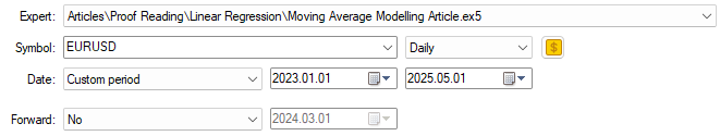
Figure 17: Our backtest days span 2 years of historical EURUSD market data

We also selected random delay settings based on real ticks to get the most accurate representation of market conditions possible. Be sure to use the same settings if you want a realistic emulation of your application’s performance.

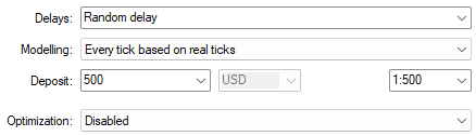
Figure 18: Selecting random delay settings for testing our trading application under realistic market conditions

In Figure 18, we can see that our application is successfully generating four independent forecasts—one for each price level of interest. It uses the filters designed in the main body of the application to open positions based on all four predictions.

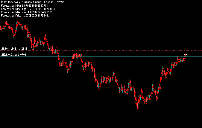
Figure 19: Backtesting our trading algorithm to test its capability to predict 4 different targets at once

I’ve included a screenshot of the terminal log to show that our application has indeed learned a matrix of coefficients. As you can see, there are four rows in the solution matrix, meaning that our application has learned one unique set of coefficients for each of the four targets we are predicting. The application learns each target independently.

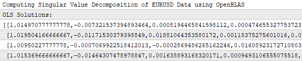
Figure 20: Our trading application learns a unique set of coefficients for each of the 4 targets we have assigned it

Moreover, our application is producing a positive trend in account balance over time. Although we would like to smooth out the irregularities in this balance, we will continue refining the system to achieve more consistent growth.

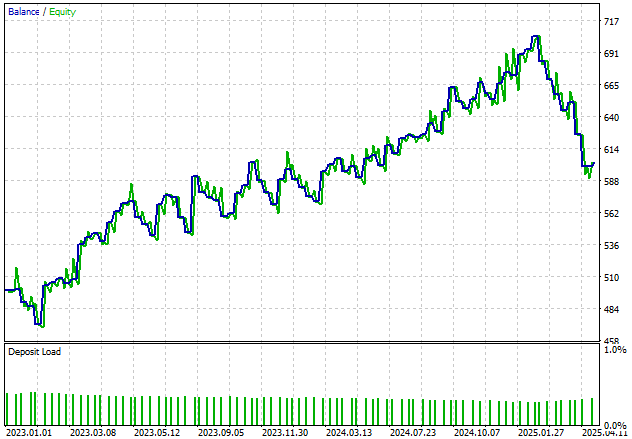
Figure 21: Visualizing the growth in our account equity curve over the 2 year back test period

When analyzing the account’s performance in detail, we find that 51% of our trades were profitable. While this is a good starting point, we aim to raise that figure to 55% or even 60% in the future. For now, we’re off to a strong start—our average profit is greater than our average loss, and our largest profit is nearly twice the size of our largest loss. This suggests the system is sound, even though we still plan to improve it.

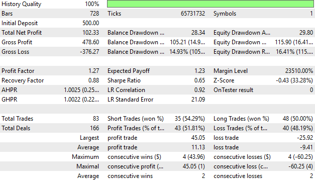
Figure 22: A detailed analysis of the performance of our trading application during our back test

Conclusion

In conclusion, this article has demonstrated to the reader the importance of a strong understanding of linear algebra concepts—and how they directly affect our ability to manipulate market data in the MetaTrader 5 terminal. Without this understanding, analyzing large volumes of market data becomes extremely difficult. By learning just a few key principles of linear algebra and seeing how they are implemented in MQL5, we gain the ability to extract insights from the market much faster and more reliably.

As we continue our discussion, we will teach the reader how to use linear algebra tools and reinterpret them in MQL5 to build numerically stable and fast trading algorithms. After reading this, the reader is now empowered to design algorithms that run in nearly constant time—allowing for rapid backtesting and improvement of their applications even if they want to predict multiple targets all at the same time.