Population optimization algorithms: Monkey algorithm (MA)

Contents:

1. Introduction
2. Algorithm
3. Test results

1. Introduction

Monkey Algorithm (MA) is a metaheuristic search algorithm. This article will describe the main components of the algorithm and present solutions for the ascent (upward movement), local jump and global jump. The algorithm was proposed by R. Zhao and W. Tang in 2007. The algorithm simulates the behavior of monkeys as they move and jump over mountains in search of food. It is assumed that the monkeys come from the fact that the higher the mountain, the more food on its top.

The area explored by the monkeys is a fitness function landscape, so the highest mountain corresponds to the solution of the problem (we consider the problem of global maximization). From its current position, each of the monkeys moves up until it reaches the top of the mountain. The climb process is designed to gradually improve the value of the target function. Then, the monkey makes a series of local jumps in a random direction in the hope of finding a higher mountain, and the upward movement is repeated. After performing a certain number of climbs and local jumps, the monkey believes that it has sufficiently explored the landscape in the vicinity of its initial position.

In order to explore a new area of the search space, the monkey performs a long global jump. The above steps are repeated a specified number of times in the algorithm parameters. The solution of the problem is declared to be the highest of the vertices found by the given population of monkeys. However, the MA spends significant computational time searching for local optimal solutions in the process of climbing. The global jump process can speed up the rate of convergence of the algorithm. The purpose of this process is to force the monkeys to find new search opportunities so as not to fall into the local search. The algorithm has such advantages as a simple structure, relatively high reliability and a good search for local optimal solutions.

MA is a new type of evolutionary algorithm that can solve many complex optimization problems characterized by non-linearity, non-differentiability and high dimensionality. The difference from other algorithms is that the time spent by the MA is mainly due to the use of the climb process to find local optimal solutions. In the next section, I will describe the main components of the algorithm, the presented solutions, the initialization, the climb, the observation and the jump.

2. Algorithm

For ease of understanding the monkey algorithm, it is reasonable to start with pseudocode.

MA algorithm pseudocode:

1. Distribute the monkeys randomly over the search space.
2. Measure the height of the monkey position.
3. Perform local jumps a fixed number of times.
4. If the new vertex obtained in step 3 is higher, then local jumps should be made from this place.
5. If the limit of the number of local jumps is exhausted and a new vertex is not found, make a global jump.
6. After step 5, repeat step 3
7. Repeat from step 2 until the stop criterion is met.

Let's analyze each point of the pseudocode in more detail.

1. At the very beginning of optimization, the search space is unknown to the monkeys. Animals are randomly located in uncharted terrain, since the position of food is equally probable in any place.

2. The process of measuring the height of the monkey position is the fulfillment of the fitness function task.

3. When making local jumps, there is a limit on their number specified in the algorithm parameters. This means that the monkey is trying to improve its current position by making small local jumps in the food area. If the newly found source of food is better, then go to step 4.

4. A new food source has been found, the local jump count is reset. Now the search for a new source of food will be made from this place.

5. If local jumps do not lead to a discovery of a better food source, the monkey concludes that the current area is fully explored and it is time to look for a new place further away. At this point, the question arises about the direction of further jumps? The idea of the algorithm is to use the center of coordinates of all monkeys, thus providing some communication - communication between monkeys in a flock: monkeys can scream loudly and, having good spatial hearing, are able to determine the exact position of their relatives. At the same time, knowing the position of their relatives (relatives will not be in places where there is no food), it is possible to approximately calculate the optimal new position of food, therefore, it is necessary to make a jump in this direction.

In the original algorithm, the monkey makes a global jump along a line passing through the center of coordinates of all monkeys and the current position of the animal. The direction of the jump can be either towards the center of coordinates, or in the opposite direction from the center. A jump in the opposite direction from the center contradicts the very logic of finding food with approximated coordinates for all monkeys, which was confirmed by my experiments with the algorithm - in fact, this is a 50% probability that there will be a distance from the global optimum.

Practice has shown that it is more profitable to jump beyond the center of coordinates than not to jump or jump in the opposite direction. The concentration of all monkeys at one point does not occur, although at first glance such logic makes this inevitable. In fact, the monkeys, having exhausted the limit of local jumps, jump further than the center, thereby rotating the position of all the monkeys in the population. If we mentally imagine higher apes obeying this algorithm, we will see a pack of animals jumping over the geometric center of the pack from time to time, while the pack itself moves towards a richer food source. This effect of "pack movement" can be clearly seen visually on the animation of the algorithm (the original algorithm does not have this effect and the results are worse).

6. Having made a global jump, the monkey begins to specify the position of the food source in the new place. The process continues until the stop criterion is met.

The whole idea of the algorithm can easily fit on a single diagram. The movement of the monkey is indicated by circles with numbers in Figure 1. Each number is a new position for the monkey. The small yellow circles represent failed local jump attempts. The number 6 indicates the position, in which the limit of local jumps has been exhausted and a new best position has not been found. Circles without numbers represent the locations of the rest of the pack. The geometric center of the pack is indicated by a small circle with coordinates (x,y).

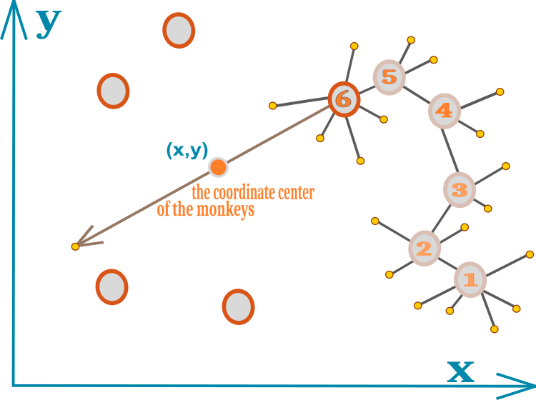
Figure 1. Schematic representation of the movement of a monkey in a pack

Let's have a look at the MA code.

It is convenient to describe a monkey in a pack with the S_Monkey structure. The structure contains the c [] array with the current coordinates, the cB [] array with the best food coordinates (it is from the position with these coordinates that local jumps occur), h and hB - the height value of the current point and the value of the highest point, respectively. lCNT — local jump counter that limits the number of attempts to improve a location.

//——————————————————————————————————————————————————————————————————————————————
struct S_Monkey
{
  double c  []; //coordinates
  double cB []; //best coordinates
  double h;     //height of the mountain
  double hB;    //best height of the mountain
  int    lCNT;  //local search counter
};
//——————————————————————————————————————————————————————————————————————————————

The C_AO_MA monkey algorithm class is no different from the algorithms discussed earlier. A pack of monkeys is represented in the class as the array of m[] structures. The declarations in the class of methods and members are small in terms of code volume. Since the algorithm is concise, there is no sorting here, unlike many other optimization algorithms. We will need arrays to set the maximum, minimum and step of the optimized parameters, as well as constant variables to pass the external parameters of the algorithm to them. Let's move on to the description of the methods that contain the main logic of MA.

//——————————————————————————————————————————————————————————————————————————————
class C_AO_MA
{
  //----------------------------------------------------------------------------
  public: S_Monkey m       []; //monkeys
  public: double rangeMax  []; //maximum search range
  public: double rangeMin  []; //minimum search range
  public: double rangeStep []; //step search
  public: double cB        []; //best coordinates
  public: double hB;           //best height of the mountain

  public: void Init (const int    coordNumberP,     //coordinates number
                     const int    monkeysNumberP,   //monkeys number
                     const double bCoefficientP,    //local search coefficient
                     const double vCoefficientP,    //jump coefficient
                     const int    jumpsNumberP);    //jumps number

  public: void Moving   ();
  public: void Revision ();

  //----------------------------------------------------------------------------
  private: int    coordNumber;       //coordinates number
  private: int    monkeysNumber;     //monkeys number

  private: double b [];              //local search coefficient
  private: double v [];              //jump coefficient
  private: double bCoefficient;      //local search coefficient
  private: double vCoefficient;      //jump coefficient
  private: double jumpsNumber;       //jumps number
  private: double cc [];             //coordinate center

  private: bool   revision;

  private: double SeInDiSp  (double In, double InMin, double InMax, double Step);
  private: double RNDfromCI (double min, double max);
  private: double Scale     (double In, double InMIN, double InMAX, double OutMIN, double OutMAX,  bool revers);
};
//——————————————————————————————————————————————————————————————————————————————

The public Init() method is for initializing the algorithm. Here we set the size of the arrays. We initialize the quality of the best territory found by the monkey with the minimum possible 'double' value, and we will do the same with the corresponding variables of the MA structure arrays.

//——————————————————————————————————————————————————————————————————————————————
void C_AO_MA::Init (const int    coordNumberP,    //coordinates number
                    const int    monkeysNumberP,  //monkeys number
                    const double bCoefficientP,   //local search coefficient
                    const double vCoefficientP,   //jump coefficient
                    const int    jumpsNumberP)    //jumps number
{
  MathSrand ((int)GetMicrosecondCount ()); // reset of the generator
  hB       = -DBL_MAX;
  revision = false;

  coordNumber   = coordNumberP;
  monkeysNumber = monkeysNumberP;
  bCoefficient  = bCoefficientP;
  vCoefficient  = vCoefficientP;
  jumpsNumber   = jumpsNumberP;

  ArrayResize (rangeMax,  coordNumber);
  ArrayResize (rangeMin,  coordNumber);
  ArrayResize (rangeStep, coordNumber);
  ArrayResize (b,         coordNumber);
  ArrayResize (v,         coordNumber);
  ArrayResize (cc,        coordNumber);

  ArrayResize (m, monkeysNumber);

  for (int i = 0; i < monkeysNumber; i++)
  {
    ArrayResize (m [i].c,  coordNumber);
    ArrayResize (m [i].cB, coordNumber);
    m [i].h    = -DBL_MAX;
    m [i].hB   = -DBL_MAX;
    m [i].lCNT = 0;
  }

  ArrayResize (cB, coordNumber);
}
//——————————————————————————————————————————————————————————————————————————————

The first public method Moving(), which is required to be executed at each iteration, implements the monkey jumping logic. At the first iteration, when the 'revision' flag is 'false', it is necessary to initialize the agents with random values in the range of coordinates of the studied space, which is equivalent to the random location of monkeys within the pack habitat. In order to reduce multiply repeated operations, such as calculating the coefficients of global and local jumps, we store the values for the corresponding coordinates (each of the coordinates can have its own dimension) in the v [] and b [] arrays. Let's reset the counter of local jumps of each monkey to zero. 

//----------------------------------------------------------------------------
if (!revision)
{
  hB = -DBL_MAX;

  for (int monk = 0; monk < monkeysNumber; monk++)
  {
    for (int c = 0; c < coordNumber; c++)
    {
      m [monk].c [c] = RNDfromCI (rangeMin [c], rangeMax [c]);
      m [monk].c [c] = SeInDiSp  (m [monk].c [c], rangeMin [c], rangeMax [c], rangeStep [c]);
      m [monk].h     = -DBL_MAX;
      m [monk].hB    = -DBL_MAX;
      m [monk].lCNT  = 0;
    }
  }

  for (int c = 0; c < coordNumber; c++)
  {
    v [c] = (rangeMax [c] - rangeMin [c]) * vCoefficient;
    b [c] = (rangeMax [c] - rangeMin [c]) * bCoefficient;
  }

  revision = true;
}

To calculate the center of coordinates of all monkeys, use the cc [] array whose dimension corresponds to the number of coordinates. The idea here is to add the coordinates of the monkeys and divide the resulting sum by the size of the population. Thus, the center of coordinates is the arithmetic average of the coordinates.

//calculate the coordinate center of the monkeys----------------------------
for (int c = 0; c < coordNumber; c++)
{
  cc [c] = 0.0;

  for (int monk = 0; monk < monkeysNumber; monk++)
  {
    cc [c] += m [monk].cB [c];
  }

  cc [c] /= monkeysNumber;
}

According to the pseudocode, if the limit of local jumps is not reached, the monkey will jump from its location in all directions with equal probability. The radius of the circle of local jumps is regulated by the coefficient of local jumps, which is recalculated in accordance with the dimension of the coordinates of the b[] array.

//local jump--------------------------------------------------------------
if (m [monk].lCNT < jumpsNumber) //local jump
{
  for (int c = 0; c < coordNumber; c++)
  {
    m [monk].c [c] = RNDfromCI (m [monk].cB [c] - b [c], m [monk].cB [c] + b [c]);      
    m [monk].c [c] = SeInDiSp (m [monk].c [c], rangeMin [c], rangeMax [c], rangeStep [c]);
  }
}

Let's move on to a very important part of the MA logic - the performance of the algorithm largely depends on the implementation of global jumps. Different authors approach this issue from different angles offering all sorts of solutions. According to the research, local jumps have little effect on the convergence of the algorithm. It is global jumps that determine the ability of the algorithm to "jump" from local extrema. My experiments with global jumps have revealed only one viable approach for this particular algorithm that improves results.

Above, we discussed the advisability of jumping towards the center of coordinates, and it is better if the end point is behind the center, and not between the center and the current coordinates. This approach applies Levy flight equations we have described in detail in the article aboutCuckoo optimization algorithm (COA).

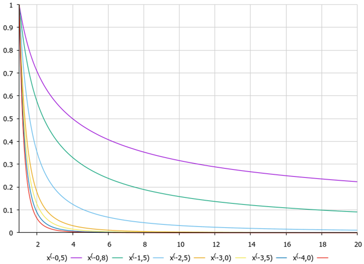
Figure 2. Graphs of the Levy flight function depending on the equation degree

Monkey coordinates are calculated using the following equation:

m [monk].c [c] = cc [c] + v [c] * pow (r2, -2.0);

where:

cc [c] — coordinate of the center of coordinates,

v [c] — coefficient of the jump radius recalculated to the dimension of the search space,

r2 — number in the range from 1 to 20.

By applying Levy's flight in this operation, we achieve a higher probability of the monkey hitting the vicinity of the center of coordinates and a lower probability of being far beyond the center. In this way, we provide a balance between research and exploitation of the search, while discovering new sources of food. If the received coordinate is beyond the lower limit of the allowable range, then the coordinate is transferred to the corresponding distance to the upper limit of the range. The same is done when going beyond the upper limit. At the end of the coordinate calculations, check the obtained value for compliance with the boundaries and the research step.

//global jump-------------------------------------------------------------
for (int c = 0; c < coordNumber; c++)
{
  r1 = RNDfromCI (0.0, 1.0);
  r1 = r1 > 0.5 ? 1.0 : -1.0;
  r2 = RNDfromCI (1.0, 20.0);

  m [monk].c [c] = cc [c] + v [c] * pow (r2, -2.0);
          
  if (m [monk].c [c] < rangeMin [c]) m [monk].c [c] = rangeMax [c] - (rangeMin [c] - m [monk].c [c]);
  if (m [monk].c [c] > rangeMax [c]) m [monk].c [c] = rangeMin [c] + (m [monk].c [c] - rangeMax [c]);
          
  m [monk].c [c] = SeInDiSp (m [monk].c [c], rangeMin [c], rangeMax [c], rangeStep [c]);
}

After making local/global jumps, increase the jump counter by one.

m [monk].lCNT++;

Revision() is the second public method called on each iteration after the fitness function has been calculated. This method updates the global solution if a better one is found. The logics of processing the results after local and global jumps differ from each other. In case of a local jump, it is necessary to check whether the current position has improved and update it (in the next iterations, jumps are made from this new place), while in case of global jumps, there is no check for improvements - new jumps will be made from this place in any case.

//——————————————————————————————————————————————————————————————————————————————
void C_AO_MA::Revision ()
{
  for (int monk = 0; monk < monkeysNumber; monk++)
  {
    if (m [monk].h > hB)
    {
      hB = m [monk].h;
      ArrayCopy (cB, m [monk].c, 0, 0, WHOLE_ARRAY);
    }

    if (m [monk].lCNT <= jumpsNumber) //local jump
    {
      if (m [monk].h > m [monk].hB)
      {
        m [monk].hB = m [monk].h;
        ArrayCopy (m [monk].cB, m [monk].c, 0, 0, WHOLE_ARRAY);
        m [monk].lCNT = 0;
      }
    }
    else //global jump
    {
      m [monk].hB = m [monk].h;
      ArrayCopy (m [monk].cB, m [monk].c, 0, 0, WHOLE_ARRAY);
      m [monk].lCNT = 0;
    }
  }
}
//——————————————————————————————————————————————————————————————————————————————

We can notice the similarity of the approaches of this algorithm with a group of swarm intelligence algorithms, such asparticle swarm (PSO) and others with a similar search strategy logic.

3. Test results

MA test stand results:

2023.02.22 19:36:21.841    Test_AO_MA (EURUSD,M1)    C_AO_MA:50;0.01;0.9;50
2023.02.22 19:36:21.841    Test_AO_MA (EURUSD,M1)    =============================
2023.02.22 19:36:26.877    Test_AO_MA (EURUSD,M1)    5 Rastrigin's; Func runs 10000 result: 64.89788419898215
2023.02.22 19:36:26.878    Test_AO_MA (EURUSD,M1)    Score: 0.80412
2023.02.22 19:36:36.734    Test_AO_MA (EURUSD,M1)    25 Rastrigin's; Func runs 10000 result: 55.57339368461394
2023.02.22 19:36:36.734    Test_AO_MA (EURUSD,M1)    Score: 0.68859
2023.02.22 19:37:34.865    Test_AO_MA (EURUSD,M1)    500 Rastrigin's; Func runs 10000 result: 41.41612351844293
2023.02.22 19:37:34.865    Test_AO_MA (EURUSD,M1)    Score: 0.51317
2023.02.22 19:37:34.865    Test_AO_MA (EURUSD,M1)    =============================
2023.02.22 19:37:39.165    Test_AO_MA (EURUSD,M1)    5 Forest's; Func runs 10000 result: 0.4307085210424681
2023.02.22 19:37:39.165    Test_AO_MA (EURUSD,M1)    Score: 0.24363
2023.02.22 19:37:49.599    Test_AO_MA (EURUSD,M1)    25 Forest's; Func runs 10000 result: 0.19875891413613866
2023.02.22 19:37:49.599    Test_AO_MA (EURUSD,M1)    Score: 0.11243
2023.02.22 19:38:47.793    Test_AO_MA (EURUSD,M1)    500 Forest's; Func runs 10000 result: 0.06286212143582881
2023.02.22 19:38:47.793    Test_AO_MA (EURUSD,M1)    Score: 0.03556
2023.02.22 19:38:47.793    Test_AO_MA (EURUSD,M1)    =============================
2023.02.22 19:38:53.947    Test_AO_MA (EURUSD,M1)    5 Megacity's; Func runs 10000 result: 2.8
2023.02.22 19:38:53.947    Test_AO_MA (EURUSD,M1)    Score: 0.23333
2023.02.22 19:39:03.336    Test_AO_MA (EURUSD,M1)    25 Megacity's; Func runs 10000 result: 0.96
2023.02.22 19:39:03.336    Test_AO_MA (EURUSD,M1)    Score: 0.08000
2023.02.22 19:40:02.068    Test_AO_MA (EURUSD,M1)    500 Megacity's; Func runs 10000 result: 0.34120000000000006
2023.02.22 19:40:02.068    Test_AO_MA (EURUSD,M1)    Score: 0.02843

Paying attention to the visualization of the algorithm on test functions, it should be noted that there are no patterns in the behavior, which is very similar to the RND algorithm. There is some small concentration of agents in local extremes, indicating attempts to refine the solution by the algorithm, but there are no obvious jams.

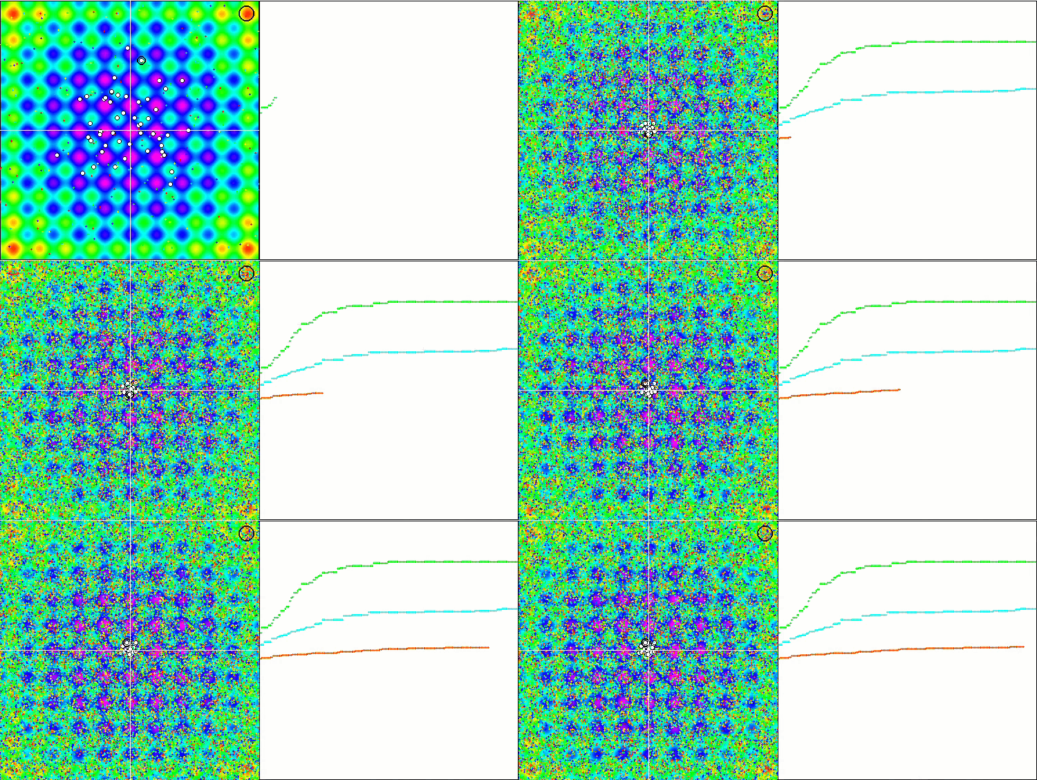
  MA on the Rastrigin test function.

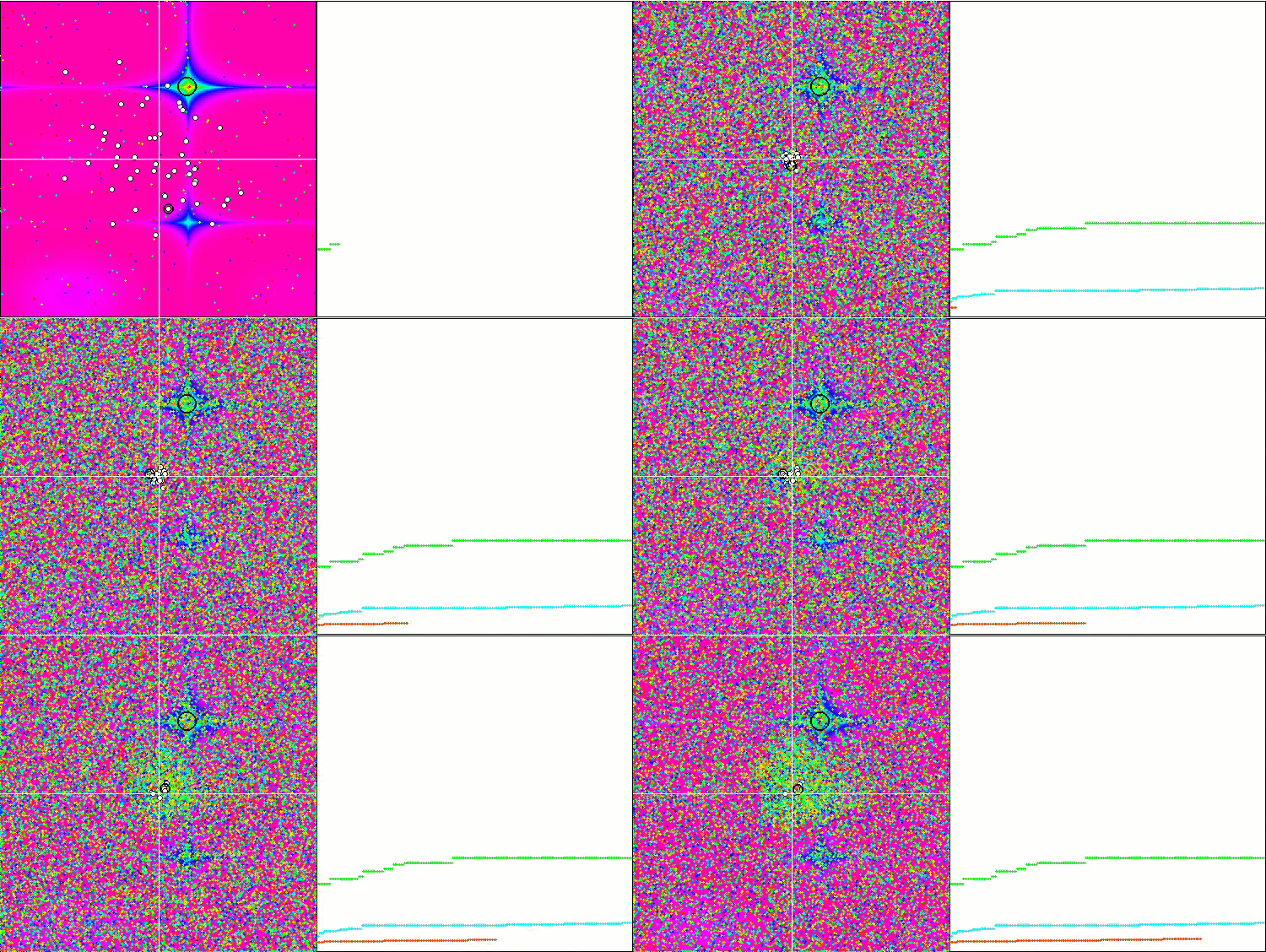
  MA on the Forest test function.

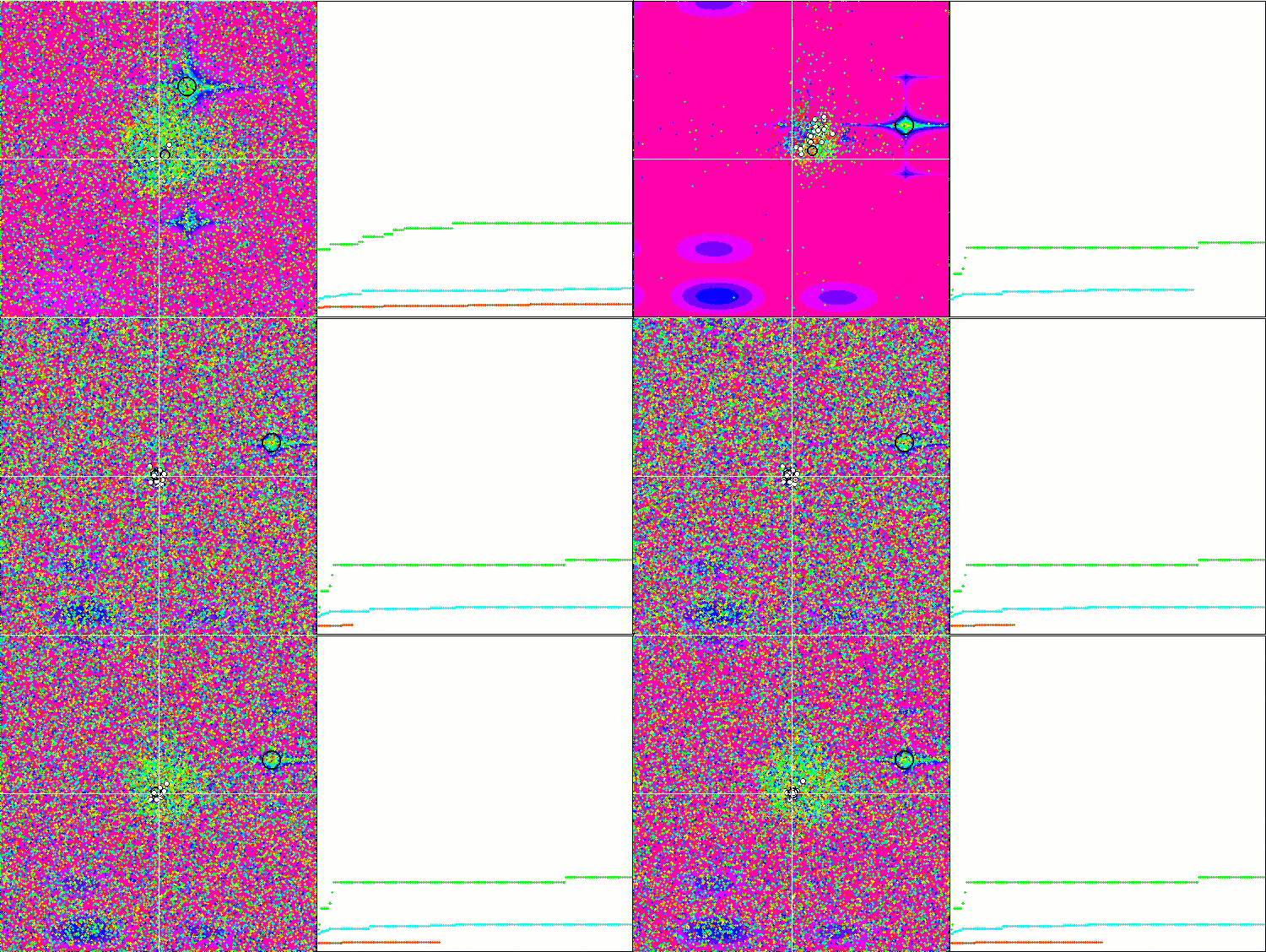
  MA on the Megacity test function.

Let's move on to the analysis of the test results. Based on the scoring results, the MA algorithm ranks at the bottom of the table between GSA and FSS. Since testing the algorithms is based on the comparative analysis principle, in which the scores of the results are relative values between the best and the worst, the emergence of an algorithm with outstanding results in one test and poor results in others sometimes causes a change in the parameters of other test participants.

But the results of MA have not caused a recalculation of any of the results of other test participants in the table. MA does not have a single test result that would be the worst, although there are algorithms with zero relative results and a higher rating (for example, GSA). Therefore, although the algorithm behaves rather modestly and the search ability is not expressed well enough, the algorithm shows stable results, which is a positive quality for optimization algorithms.

AO	Description	Rastrigin			Rastrigin final	Forest			Forest final	Megacity (discrete)			Megacity final	Final result
		10 params (5 F)	50 params (25 F)	1000 params (500 F)		10 params (5 F)	50 params (25 F)	1000 params (500 F)		10 params (5 F)	50 params (25 F)	1000 params (500 F)
HS	harmony search	1.00000	1.00000	0.57048	2.57048	1.00000	0.98931	0.57917	2.56848	1.00000	1.00000	1.00000	3.00000	100.000
ACOm	ant colony optimization M	0.34724	0.18876	0.20182	0.73782	0.85966	1.00000	1.00000	2.85966	1.00000	0.88484	0.13497	2.01981	68.094
IWO	invasive weed optimization	0.96140	0.70405	0.35295	2.01840	0.68718	0.46349	0.41071	1.56138	0.75912	0.39732	0.80145	1.95789	67.087
COAm	cuckoo optimization algorithm M	0.92701	0.49111	0.30792	1.72604	0.55451	0.34034	0.21362	1.10847	0.67153	0.30326	0.41127	1.38606	50.422
FAm	firefly algorithm M	0.60020	0.35662	0.20290	1.15972	0.47632	0.42299	0.64360	1.54291	0.21167	0.25143	0.84884	1.31194	47.816
BA	bat algorithm	0.40658	0.66918	1.00000	2.07576	0.15275	0.17477	0.33595	0.66347	0.15329	0.06334	0.41821	0.63484	39.711
ABC	artificial bee colony	0.78424	0.34335	0.24656	1.37415	0.50591	0.21455	0.17249	0.89295	0.47444	0.23609	0.33526	1.04579	38.937
BFO	bacterial foraging optimization	0.67422	0.32496	0.13988	1.13906	0.35462	0.26623	0.26695	0.88780	0.42336	0.30519	0.45578	1.18433	37.651
GSA	gravitational search algorithm	0.70396	0.47456	0.00000	1.17852	0.26854	0.36416	0.42921	1.06191	0.51095	0.32436	0.00000	0.83531	35.937
MA	monkey algorithm	0.33300	0.35107	0.17340	0.85747	0.03684	0.07891	0.11546	0.23121	0.05838	0.00383	0.25809	0.32030	14.848
FSS	fish school search	0.46965	0.26591	0.13383	0.86939	0.06711	0.05013	0.08423	0.20147	0.00000	0.00959	0.19942	0.20901	13.215
PSO	particle swarm optimisation	0.20515	0.08606	0.08448	0.37569	0.13192	0.10486	0.28099	0.51777	0.08028	0.21100	0.04711	0.33839	10.208
RND	random	0.16881	0.10226	0.09495	0.36602	0.07413	0.04810	0.06094	0.18317	0.00000	0.00000	0.11850	0.11850	5.469
GWO	grey wolf optimizer	0.00000	0.00000	0.02672	0.02672	0.00000	0.00000	0.00000	0.00000	0.18977	0.03645	0.06156	0.28778	1.000

Summary

The classical MA algorithm basically consists in using the climb process to find local optimal solutions. The climb step plays a decisive role in the accuracy of the approximation of the local solution. The smaller the climb step for local jumps, the higher the accuracy of the solution, but more iterations are required to find the global optimum. To reduce computation time by reducing the number of iterations, many researchers recommend using other optimization methods at the initial stages of optimization, such as ABC, COA, IWO, and use MA to refine the global solution. I do not agree with this approach. I believe, it is more expedient to immediately use the described algorithms instead of MA, although MA has the development potential making it a good object for further experiments and study. 

The Monkey Algorithm is a population-based algorithm that has its roots in nature. Like many other metaheuristic algorithms, this algorithm is evolutionary and is able to solve a number of optimization problems, including non-linearity, non-differentiability and high dimensionality of the search space with a high convergence rate. Another advantage of the monkey algorithm is that this algorithm is controlled by a small number of parameters, making it fairly easy to implement. Despite the stability of the results, the low rate of convergence does not allow recommending the monkey algorithm for solving problems with high computational complexity, since it requires a significant number of iterations. There are many other algorithms doing the same work in a shorter time (number of iterations).

Despite my numerous experiments, the classical version of the algorithm could not get higher than the third from the bottom line of the rating table, got stuck in local extremes and worked extremely poorly on discrete functions. I did not have particular desire to write an article about it, so I made attempts to improve it. One of these attempts showed some improvements in convergence indicators and increased the stability of the results by using probability bias in global jumps, as well as revising the principle of global jumps themselves. Many MA researchers point out the need to modernize the algorithm, so there are many modifications to the monkey algorithm. It was not my intention to consider all kinds of modifications of MA, because the algorithm itself is not outstanding, rather it is a variation of the particle swarm (PSO). The result of the experiments was the final version of the algorithm given in this article without the additional 'm' (modified) marking.

The histogram of the algorithm test results is provided below.

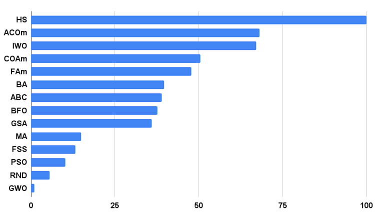
Figure 3. Histogram of the test results of the algorithms

MA pros and cons:

Pros:
1. Easy implementation.
2. Good scalability despite low convergence rate.
3. Good performance on discrete functions.
4. Small number of external parameters.

Cons:
1. Low convergence rate.
2. Requires a large number of iterations for a search.
3. Low overall efficiency.

Each article features an archive that contains updated current versions of the algorithm codes for all previous articles. The article is based on the accumulated experience of the author and represents his personal opinion. The conclusions and judgments are based on the experiments.