Population optimization algorithms: Simulated Isotropic Annealing (SIA) algorithm. Part II

Contents

1. Introduction
2. Algorithm
3. Test results

1. Introduction

In the first part, we considered the conventional version of the Simulated Annealing (SA) algorithm. The algorithm is based on three main concepts: applying randomness, making worse decisions and gradually reducing the likelihood of making worse decisions. Applying randomness allows exploring different regions of the search space and avoid getting stuck in local optima. Accepting worse decisions with some probability allows the algorithm to temporarily "jump" out of local optima and look for better solutions elsewhere in the search space, allowing it to first explore the search space more broadly and then focus on improving the solution.

The idea of the SA algorithm is based on the metal annealing analogy. The preheated metal gradually cools, which leads to a change in its structure. Similarly, the simulated annealing algorithm starts with a high temperature (high probability of making a worse decision) and gradually decreases the temperature (decreases the probability of making a worse decision), which is supposed to help the algorithm converge to the optimal solution.

The algorithm begins its work with an initial solution, which can be random or obtained from previous iterations. Then it applies operations to change the state of the solution, which can be random or controlled, to obtain a new state, even if it is worse than the current one. The probability of making a worse decision is determined by the "cooling" function, which reduces the probability of making a worse decision over time.

Several simple equations are used to describe the simulated annealing. The equation for calculating the change in energy allows us to determine the difference in the values of the fitness function at two successive iterations. The equation for calculating the probability of making a worse decision determines the probability of accepting a new state taking into account the difference in energy and current temperature.

The important parameters that need to be adjusted when using the simulated annealing algorithm are the initial temperature and the cooling ratio. Setting these parameters can have a significant impact on the performance and quality of the solution and is one of the weaknesses of the algorithm - the difficulty in choosing parameters due to their unobvious impact on performance. In addition, both of these parameters mutually influence each other: an increase in temperature can almost equally be replaced by a decrease in the temperature reduction ratio.

In the first part of the article, we identified the main problems of the algorithm:

• Parameter tuning: Parameters of the SA algorithm, such as initial temperature and cooling coefficient, can significantly affect its performance and efficiency. Setting these parameters can be challenging and requires experimentation to achieve optimal values.

• The issue of getting stuck in local extrema: To overcome it, we can apply various strategies, such as choosing the most appropriate distribution of the random variable when generating new solutions in combination with the existing algorithm strategy tools, as well as considering possible solutions to improve the combinatorial capabilities.

• Improved convergence speed: To speed up convergence, modifications to the cooling function can be applied to allow the system temperature to be reduced more quickly (or with a different form of cooling function). We can also revise the methods for selecting the next state in the algorithm, which take into account information about previously passed states.

• Improving the efficiency of the SA algorithm with a large number of variables: This is one of the most difficult problems for the vast majority of algorithms. As the number of variables increases, the complexity of the search space grows much faster than can be taken into account using special methods in search strategies. 

One of the main problems in multidimensional spaces is the combinatorial explosion of possible combinations of variables. As the number of variables increases, the number of possible system states that need to be explored increases exponentially. This causes optimization algorithms to face the problem of spatial complexity.

Spatial complexity means that the size of the search space grows exponentially as the number of variables increases. For example, if we have 10 variables, each of which can take 10 values, then the total number of possible combinations is equal to 10^10, which is equal to 10 billion, despite the fact that we only have 10 thousand attempts (the number of fitness function runs). Finding the optimal solution among so many combinations becomes an extremely difficult task. Separately, it is worth noting that in our tests we optimize function parameters with a step of 0. This means incredibly difficult conditions for the algorithms. Those of them that cope satisfactorily on such complex test problems will be almost guaranteed to work better on less complex ones real problems (all other things being equal).

2. Algorithm

The simulated annealing algorithm is so simple that it is truly difficult to imagine how it could be improved further. It is like turning a glass of water into an enchanting wine — an act of magic. Indeed, what can be improved if the generation of new values is evenly distributed, and the idea of making the worst decision completely violates the usual logic of constructing optimization algorithms?

Let's have a look at the printout of the results from the previous article to visually compare subsequent experimental results with the initial reference result of the original simulated annealing (SA) algorithm:

C_AO_SA:50:1000.0:0.1:0.2
=============================
5 Rastrigin's; Func runs 10000 result: 65.78409729002105
Score: 0.81510
25 Rastrigin's; Func runs 10000 result: 52.25447043222567
Score: 0.64746
500 Rastrigin's; Func runs 10000 result: 40.40159931988021
Score: 0.50060
=============================
5 Forest's; Func runs 10000 result: 0.5814827554067439
Score: 0.32892
25 Forest's; Func runs 10000 result: 0.23156336186841173
Score: 0.13098
500 Forest's; Func runs 10000 result: 0.06760002887601002
Score: 0.03824
=============================
5 Megacity's; Func runs 10000 result: 2.92
Score: 0.24333
25 Megacity's; Func runs 10000 result: 1.256
Score: 0.10467
500 Megacity's; Func runs 10000 result: 0.33840000000000003
Score: 0.02820
=============================
All score: 2.83750

Let's try to improve the results by replacing the uniform distribution of random variables with a normal one when generating new states of the system.

We will use the simulated annealing algorithm class as the basis for the new SIA algorithm, so we will not provide a description of the methods and functionality of this class, since everything has already been done in the first part of the article.

Then, we can use the inverse function method to generate a random number with a normal distribution. Suppose that we want to generate an "x" number with a normal distribution, mu (mean) and sigma (standard deviation). Then we can use the following equation:

x = z0 * sigma + mu

where:

• z0 - calculate using the equation:

z0 = sqrt (-2 * log (u1)) * cos(2 * Pi * u2)

where:

• u1* - random number in the range (0.0;1.0] (here 'min' is not included in the range)
  

• u2** - random number in the range [0.0;1.0]

• * and ** - two independent random numbers with uniform distribution
  

In the previous article, we added a diffusion ratio parameter to the SA algorithm, which limits the range of random number generation. It is in this area that we should generate random numbers.

Let's write the C_AO_SIA class method that simulates diffusion - "Diffusion". The method generates a random number with a normal distribution of up to two standard deviations. We wrap values that go beyond these boundaries "inside" without losing the shape of the distribution (we will look at it in more detail in one of the following articles).

Knowing the value of the standard deviation (sigma), we can translate this range of values into our required range simulating diffusion. For this, we use the Scale scaling function.

//——————————————————————————————————————————————————————————————————————————————
double C_AO_SIA::Diffusion (const double value, const double rMin, const double rMax, const double step)
{
  double logN = 0.0;
  double u1   = RNDfromCI (0.0, 1.0);
  double u2   = RNDfromCI (0.0, 1.0);

  logN = u1 <= 0.0 ? 0.000000000000001 : u1;

  double z0 = sqrt (-2 * log (logN))* cos (2 * M_PI * u2);

  double sigma = 2.0;//Sigma > 8.583864105157389 ? 8.583864105157389 : Sigma;

  if (z0 >=  sigma) z0 = RNDfromCI (0.0,    sigma);
  if (z0 <= -sigma) z0 = RNDfromCI (-sigma, 0.0);

  double dist = d * (rMax - rMin);

  if (z0 >= 0.0) return Scale (z0, 0.0,    sigma, value,        value + dist, false);
  else           return Scale (z0, -sigma, 0.0,   value - dist, value,        false);
}
//——————————————————————————————————————————————————————————————————————————————

In the Moving method, we will use the Diffusion method like this:

for (int i = 0; i < popSize; i++)
{
   for (int c = 0; c < coords; c++)
   {
     a [i].c [c] = Diffusion (a [i].c [c], rangeMin [c], rangeMax [c], rangeStep [c]);
     a [i].c [c] = SeInDiSp  (a [i].c [c], rangeMin [c], rangeMax [c], rangeStep [c]);
   } 
}

After running the tests with the changes made (replacing the uniform distribution with a normal distribution), we got the following results:

C_AO_SIA:50:1000.0:0.1:0.2
=============================
5 Rastrigin's; Func runs 10000 result: 60.999013617749895
Score: 0.75581
25 Rastrigin's; Func runs 10000 result: 47.993562806349246
Score: 0.59467
500 Rastrigin's; Func runs 10000 result: 40.00575378955945
Score: 0.49569
=============================
5 Forest's; Func runs 10000 result: 0.41673083215719087
Score: 0.23572
25 Forest's; Func runs 10000 result: 0.16700842421505407
Score: 0.09447
500 Forest's; Func runs 10000 result: 0.049538421252065555
Score: 0.02802
=============================
5 Megacity's; Func runs 10000 result: 2.7600000000000002
Score: 0.23000
25 Megacity's; Func runs 10000 result: 0.9039999999999999
Score: 0.07533
500 Megacity's; Func runs 10000 result: 0.28
Score: 0.02333
=============================
All score: 2.53305

When we change the distribution of a random variable in a simulated annealing algorithm, as in any other algorithm, this will certainly affect its operation and results. The original equation of the algorithm uses a uniform distribution to generate random steps to explore the solution space. This distribution ensures equal probabilities for all possible steps.

When we replaced the uniform distribution with the normal distribution, the probabilistic properties of the algorithm changed. A normal distribution peaks around the mean and decreases as it moves away from the mean. This means that random steps generated using a normal distribution will be concentrated around the mean. Steps far from the mean are less likely to occur. In our case, the "average value" is the original coordinate value we want to improve.

This change in distribution obviously leads to less varied steps in exploring the solution space. The algorithm appears to become more local and less able to explore more distant or less likely regions of the solution space.

The tests above show that in this case the use of the normal distribution led to a slight but statistically significant deterioration in the final results compared to a uniformly distributed random variable (as reflected in the first part of the article). These results were obtained using two standard deviations, and increasing the sigma (standard deviation) value results in a further statistically significant deterioration in the results.

From this we conclude that changing the shape of the distribution to a more acute one worsens the results in this particular case.

Now that we have realized that "sharpening" the shape of the distribution in the original algorithm is not beneficial, let's look at another approach. Let us assume that in the original algorithm, molecules in the metal, or, one might say, entire crystals within the diffusion zone, do not have enough opportunity to exchange energy in order to distribute it evenly throughout the entire volume of the metal. In this case, we can propose the following idea: allow the crystals to exchange molecules while exchanging energy.

The exchange of molecules between crystals with different energies will allow the transfer of coordinates between agents. Thus, the molecules will become some kind of energy carriers capable of smoothing out the energy distribution throughout the entire volume of the metal. As a result of this interaction between the crystal lattice and molecules, energy will be more evenly distributed, which will allow a more stable and optimal system configuration to be achieved. In other words, we will try to increase the isotropy in the metal structure.

Isotropy is the property of an object or system to retain the same characteristics or properties in all directions. In simpler terms, an object or system is isotropic if it looks and behaves the same in every direction. Thus, isotropy implies that there is no preferred direction or orientation, and the object or system is considered the same or homogeneous in all directions.

To simulate the equalization of properties in the metal in all directions (increasing isotropy), we will need to make changes to the Moving method.

The logic of the code is as follows: iteration is performed over each element of the "popSize" population and each "coords" coordinate:

• a random integer "r" is generated in the range from 0 to "popSize" using the RNDfromCI function, thereby randomly selecting an agent in the population
  
• check the condition: if the value of the fitness function of the selected agent is greater than the fitness value of the agent being changed, then we copy the coordinate of the best one, otherwise the coordinate of the agent does not change
  
• generates a random "rnd" number in the range [-0.1;0.1] using the RNDfromCI function
• the coordinate value is updated by adding to it the product of "rnd", (rangeMax[c] - rangeMin[c]) and "d", i.e. adding a random increment in the diffusion range
• check the resulting coordinate using the SeInDiSp function so that it is within the permissible range and with the required step
  

int    r   = 0;
double rnd = 0.0;

for (int i = 0; i < popSize; i++)
{
  for (int c = 0; c < coords; c++)
  {
      
    r = (int)RNDfromCI (0, popSize);
    if (r >= popSize) r = popSize - 1;

    if (a [r].fPrev > a [i].fPrev)
    {
      a [i].c [c] = a [r].cPrev [c];
    }
    else
    {
      a [i].c [c] = a [i].cPrev [c];
    }
      
    rnd = RNDfromCI (-0.1, 0.1);
    a [i].c [c] = a [i].c [c] + rnd * (rangeMax [c] - rangeMin [c]) * d;
    a [i].c [c] = SeInDiSp (a [i].c [c], rangeMin [c], rangeMax [c], rangeStep [c]);
  }
}

Results of annealing with the same parameters with a uniform distribution and isotropy:

C_AO_SIA:50:1000.0:0.1:0.1
=============================
5 Rastrigin's; Func runs 10000 result: 80.52391137534615
Score: 0.99774
25 Rastrigin's; Func runs 10000 result: 77.70887543197314
Score: 0.96286
500 Rastrigin's; Func runs 10000 result: 57.43358792423487
Score: 0.71163
=============================
5 Forest's; Func runs 10000 result: 1.5720970326889474
Score: 0.88926
25 Forest's; Func runs 10000 result: 1.0118351454323513
Score: 0.57234
500 Forest's; Func runs 10000 result: 0.3391169587652742
Score: 0.19182
=============================
5 Megacity's; Func runs 10000 result: 6.76
Score: 0.56333
25 Megacity's; Func runs 10000 result: 5.263999999999999
Score: 0.43867
500 Megacity's; Func runs 10000 result: 1.4908
Score: 0.12423
=============================
All score: 5.45188

The use of increasing isotropy, in which molecules are exchanged between crystals with different energies, has led to a significant improvement in the algorithm results. This is a claim to leadership.

Conclusions that can be drawn based on the described process:

• Transfer of coordinates between agents: the exchange of molecules between crystals with different energies allows the transfer of coordinate information between agents in the algorithm. This contributes to a more efficient and faster search for the optimal solution, since information about good solutions is transmitted to other agents
• Smoothing of energy distribution: the process of exchange of molecules between crystals with different energies allows to smooth out the energy distribution throughout the entire metal volume. This means that energy will be more evenly distributed, which helps avoid local minima and achieve a more stable and optimal system configuration

Now, after significantly improving the results by adding isotropy, let's try adding the normal distribution again (first we perform the operation of increasing isotropy and adding the increment with the normal distribution to the resulting values).

Annealing results with added isotropy enhancement + normal distribution:

C_AO_SIA:50:1000.0:0.1:0.05
=============================
5 Rastrigin's; Func runs 10000 result: 78.39172420614801
Score: 0.97132
25 Rastrigin's; Func runs 10000 result: 66.41980717898778
Score: 0.82298
500 Rastrigin's; Func runs 10000 result: 47.62039509425823
Score: 0.59004
=============================
5 Forest's; Func runs 10000 result: 1.243327107341557
Score: 0.70329
25 Forest's; Func runs 10000 result: 0.7588262864735575
Score: 0.42923
500 Forest's; Func runs 10000 result: 0.13750740782669305
Score: 0.07778
=============================
5 Megacity's; Func runs 10000 result: 6.8
Score: 0.56667
25 Megacity's; Func runs 10000 result: 2.776
Score: 0.23133
500 Megacity's; Func runs 10000 result: 0.46959999999999996
Score: 0.03913
=============================
All score: 4.43177

The results have deteriorated significantly.

Generating normally distributed increments in the simulated annealing algorithm have not brought any improvement. Can a normally distributed increment provide the expected effect after applying isotropy enhancement? Expectations have not been confirmed. This can be explained by the fact that after isotropy enhancement is applied, the still uniform distribution allows for a more uniform exploration of the solution space, allowing the algorithm to explore different regions without strongly biasing preferences. An attempt to refine the existing coordinates using the normal distribution has been unsuccessful. This limits a broader exploration of the algorithm areas.

Let's carry out the last experiment in order to finally draw conclusions in favor of a uniform distribution of increments of the random variable after applying an increase in isotropy. We will explore the neighborhood of known coordinates even more accurately by using the quadratic distribution for this. If a uniformly distributed random variable is raised to the second power, the resulting distribution is called the squared distribution of the random variable or the quadratic distribution.

Results of the simulated annealing algorithm with the same parameters including isotropy enhancement + sharp quadratic distribution:

C_AO_SIA:50:1000.0:0.1:0.2
=============================
5 Rastrigin's; Func runs 10000 result: 70.23675927985173
Score: 0.87027
25 Rastrigin's; Func runs 10000 result: 56.86176837508631
Score: 0.70455
500 Rastrigin's; Func runs 10000 result: 43.100825665204596
Score: 0.53404
=============================
5 Forest's; Func runs 10000 result: 0.9361317757226002
Score: 0.52952
25 Forest's; Func runs 10000 result: 0.25320813586138297
Score: 0.14323
500 Forest's; Func runs 10000 result: 0.0570263375476293
Score: 0.03226
=============================
5 Megacity's; Func runs 10000 result: 4.2
Score: 0.35000
25 Megacity's; Func runs 10000 result: 1.296
Score: 0.10800
500 Megacity's; Func runs 10000 result: 0.2976
Score: 0.02480
=============================
All score: 3.29667

Squaring a uniformly distributed random variable also has not provided a positive effect. The decline in performance was even stronger than using the normal distribution.

Now, let’s get rid of one more drawback of the simulated annealing algorithm - the difficulty in choosing settings and the combination of temperature and temperature reduction ratio, since both of these parameters mutually influence each other. In order to link these two parameters together, combine the temperature reduction function and the function of probabilistic worse decision-making. Let's apply the hyperbolic arc cosine function:

(1 - delta) * (acosh (-(x^3 - 3))) / 1,765

where:

• delta - the difference between the values of the fitness function at the last two iterations, normalized to the range [0.0;1.0]
• x - normalized algorithm epoch steps

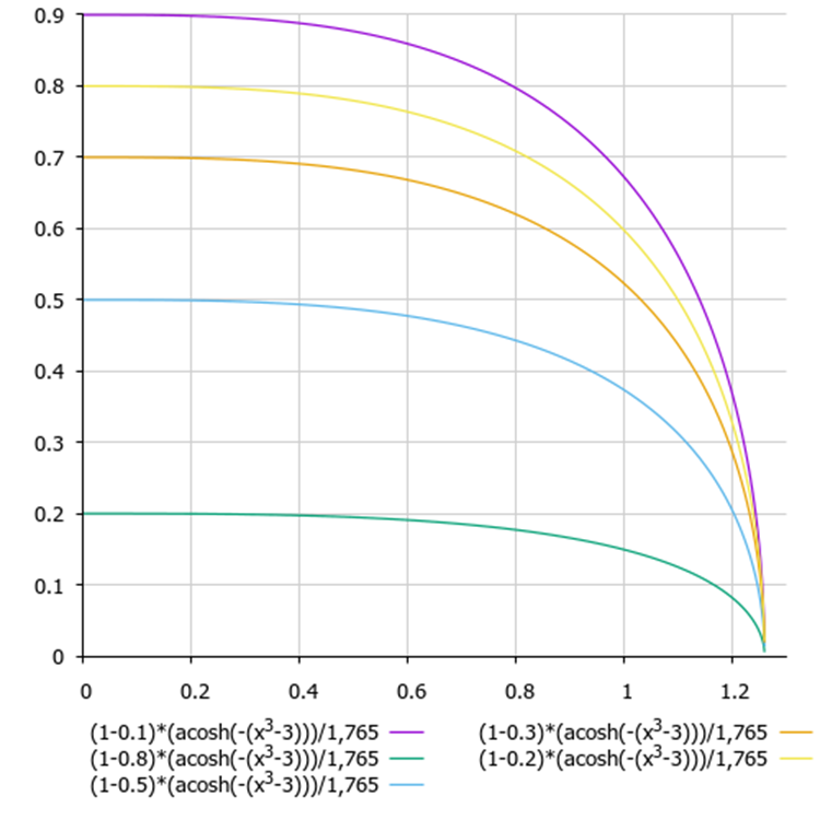
Figure 1. Graph of the dependence of making the worst decision on the energy difference and the number of the current epoch (y - energy difference, x - epochs)

3. Test results

SIA test stand results:

C_AO_SIA:100:0.01:0.1
=============================
5 Rastrigin's; Func runs 10000 result: 80.49732910930824
Score: 0.99741
25 Rastrigin's; Func runs 10000 result: 78.48411039606445
Score: 0.97246
500 Rastrigin's; Func runs 10000 result: 56.26829697982381
Score: 0.69720
=============================
5 Forest's; Func runs 10000 result: 1.6491133508905373
Score: 0.93282
25 Forest's; Func runs 10000 result: 1.3608802086313785
Score: 0.76978
500 Forest's; Func runs 10000 result: 0.31584037846210056
Score: 0.17866
=============================
5 Megacity's; Func runs 10000 result: 8.6
Score: 0.71667
25 Megacity's; Func runs 10000 result: 6.152
Score: 0.51267
500 Megacity's; Func runs 10000 result: 1.0544
Score: 0.08787
=============================
All score: 5.86552

The results are impressive. Besides, the number of parameters have decreased by one.

Visualization of the algorithm operation demonstrates a clear division into separate clusters of agents with all significant local extrema covered. The image resembles the actual crystallization of solidifying metal. We can clearly see the excellent convergence on all tests, including the ones with many variables.

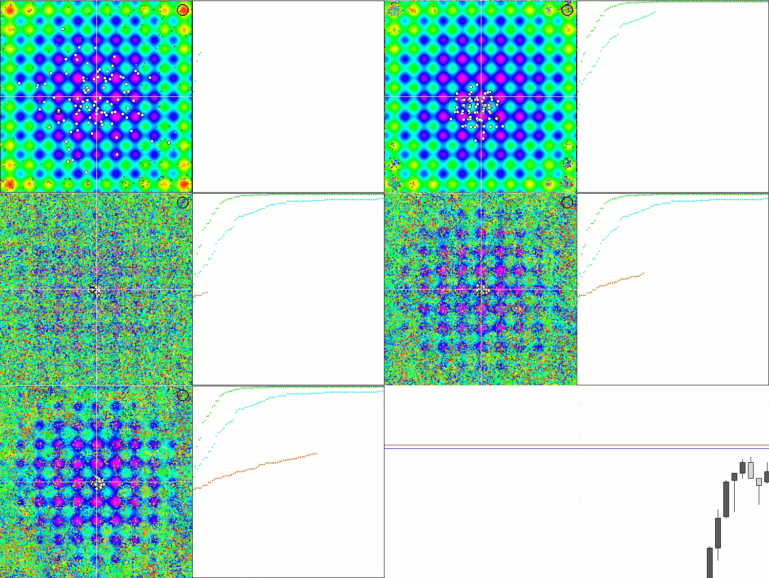
SIA on the Rastrigin test function

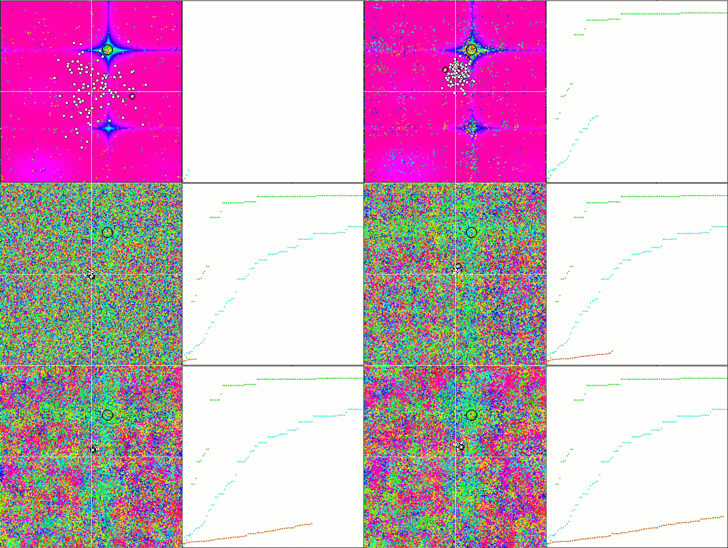
SIA on the Forest test function

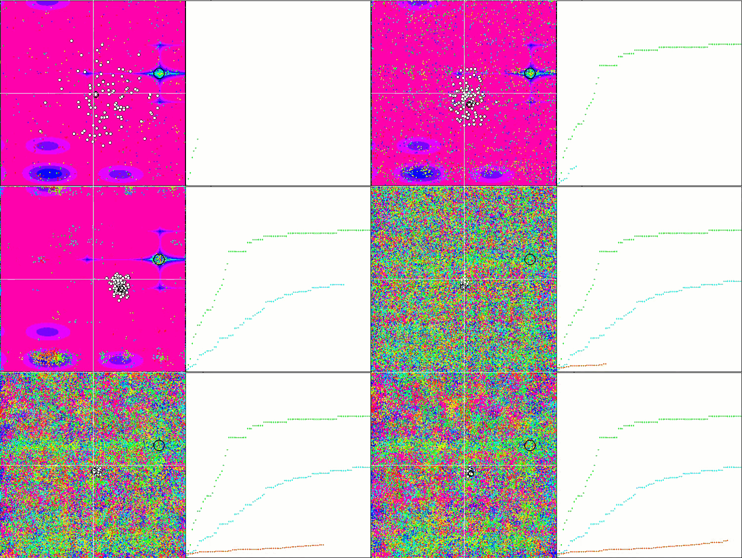
  SIA on the Megacity test function

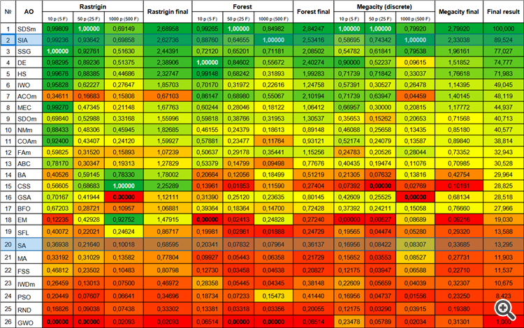
The new algorithm for simulating isotropic annealing (SIA, 2023) took second place in the rating table replacing SDSm in two of the most difficult tests (acute Forest and discrete Megacity with 1000 variables).

#	AO	Description	Rastrigin			Rastrigin final	Forest			Forest final	Megacity (discrete)			Megacity final	Final result
			10 p (5 F)	50 p (25 F)	1000 p (500 F)		10 p (5 F)	50 p (25 F)	1000 p (500 F)		10 p (5 F)	50 p (25 F)	1000 p (500 F)
1	SDSm	stochastic diffusion search M	0.99809	1.00000	0.69149	2.68958	0.99265	1.00000	0,84982	2,84247	1.00000	1.00000	0,79920	2,79920	100.000
2	SIA	simulated isotropic annealing	0.99236	0.93642	0.69858	2.62736	0.88760	0.64655	1.00000	2.53416	0.58695	0.74342	1.00000	2.33038	89.524
3	SSG	saplings sowing and growing	1.00000	0.92761	0.51630	2.44391	0.72120	0.65201	0.71181	2.08502	0.54782	0.61841	0.79538	1.96161	77.027
4	DE	differential evolution	0.98295	0.89236	0.51375	2.38906	1.00000	0.84602	0.55672	2.40274	0.90000	0.52237	0.09615	1.51852	74.777
5	HS	harmony search	0.99676	0.88385	0.44686	2.32747	0.99148	0.68242	0.31893	1.99283	0.71739	0.71842	0.33037	1.76618	71.983
6	IWO	invasive weed optimization	0.95828	0.62227	0.27647	1.85703	0.70170	0.31972	0.22616	1.24758	0.57391	0.30527	0.26478	1.14395	49.045
7	ACOm	ant colony optimization M	0.34611	0.16683	0.15808	0.67103	0.86147	0.68980	0.55067	2.10194	0.71739	0.63947	0.04459	1.40145	48.119
8	MEC	mind evolutionary computation	0.99270	0.47345	0.21148	1.67763	0.60244	0.28046	0.18122	1.06412	0.66957	0.30000	0.20815	1.17772	44.937
9	SDOm	spiral dynamics optimization M	0.69840	0.52988	0.33168	1.55996	0.59818	0.38766	0.31953	1.30537	0.35653	0.15262	0.20653	0.71568	40.713
10	NMm	Nelder-Mead method M	0.88433	0.48306	0.45945	1.82685	0.46155	0.24379	0.18613	0.89148	0.46088	0.25658	0.13435	0.85180	40.577
11	COAm	cuckoo optimization algorithm M	0.92400	0.43407	0.24120	1.59927	0.57881	0.23477	0.11764	0.93121	0.52174	0.24079	0.13587	0.89840	38.814
12	FAm	firefly algorithm M	0.59825	0.31520	0.15893	1.07239	0.50637	0.29178	0.35441	1.15256	0.24783	0.20526	0.28044	0.73352	32.943
13	ABC	artificial bee colony	0.78170	0.30347	0.19313	1.27829	0.53379	0.14799	0.09498	0.77676	0.40435	0.19474	0.11076	0.70985	30.528
14	BA	bat algorithm	0.40526	0.59145	0.78330	1.78002	0.20664	0.12056	0.18499	0.51219	0.21305	0.07632	0.13816	0.42754	29.964
15	CSS	charged system search	0.56605	0.68683	1.00000	2.25289	0.13961	0.01853	0.11590	0.27404	0.07392	0.00000	0.02769	0.10161	28.825
16	GSA	gravitational search algorithm	0.70167	0.41944	0.00000	1.12111	0.31390	0.25120	0.23635	0.80145	0.42609	0.25525	0.00000	0.68134	28.518
17	BFO	bacterial foraging optimization	0.67203	0.28721	0.10957	1.06881	0.39364	0.18364	0.14700	0.72428	0.37392	0.24211	0.15058	0.76660	27.966
18	EM	electroMagnetism-like algorithm	0.12235	0.42928	0.92752	1.47915	0.00000	0.02413	0.24828	0.27240	0.00000	0.00527	0.08689	0.09216	19.030
19	SFL	shuffled frog-leaping	0.40072	0.22021	0.24624	0.86717	0.19981	0.02861	0.01888	0.24729	0.19565	0.04474	0.05280	0.29320	13.588
20	SA	simulated annealing	0.36938	0.21640	0.10018	0.68595	0.20341	0.07832	0.07964	0.36137	0.16956	0.08422	0.08307	0.33685	13.295
21	MA	monkey algorithm	0.33192	0.31029	0.13582	0.77804	0.09927	0.05443	0.06358	0.21729	0.15652	0.03553	0.08527	0.27731	11.903
22	FSS	fish school search	0.46812	0.23502	0.10483	0.80798	0.12730	0.03458	0.04638	0.20827	0.12175	0.03947	0.06588	0.22710	11.537
23	IWDm	intelligent water drops M	0.26459	0.13013	0.07500	0.46972	0.28358	0.05445	0.04345	0.38148	0.22609	0.05659	0.04039	0.32307	10.675
24	PSO	particle swarm optimisation	0.20449	0.07607	0.06641	0.34696	0.18734	0.07233	0.15473	0.41440	0.16956	0.04737	0.01556	0.23250	8.423
25	RND	random	0.16826	0.09038	0.07438	0.33302	0.13381	0.03318	0.03356	0.20055	0.12175	0.03290	0.03915	0.19380	5.097
26	GWO	grey wolf optimizer	0.00000	0.00000	0.02093	0.02093	0.06514	0.00000	0.00000	0.06514	0.23478	0.05789	0.02034	0.31301	1.000

Summary

Based on the experiments performed and analysis of the results, we can draw the following conclusions:

1. The new Simulated Isotropic Annealing (SIA) algorithm demonstrates impressive results in optimizing functions with multiple variables. This indicates the efficiency of the algorithm in finding optimal solutions in high-dimensional spaces.
2. The algorithm shows particularly good results on functions with sharp and discrete features. This may be due to the fact that SIA allows us to uniformly explore the solution space and find optimal points even in complex and irregular regions.
3. Overall, the new SIA algorithm is a powerful optimization tool. Thanks to the successful combination of search strategies, the algorithm has qualitatively new properties and demonstrates high efficiency in finding optimal solutions.

In the new SIA algorithm, in addition to the population size, there are only two parameters (temperature and diffusion ratio) instead of three as in SA. In addition, now the temperature parameter is very easy to understand and is expressed in parts of some abstract temperature and is equal to 0.01 by default.

Based on the research and analysis of the results, we can confidently recommend the SIA algorithm for use in training neural networks and in trading problems with many parameters and complex combinatorics problems.

Figure 2. Color gradation of algorithms according to relevant tests

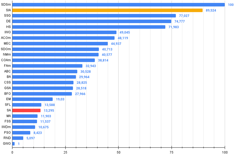
Figure 3. The histogram of algorithm test results (on a scale from 0 to 100, the more the better,

the archive contains the script for calculating the rating table using the method applied in the article).

SIA pros and cons:

Advantages:

1. Minimum number of external parameters.
2. High efficiency in solving a variety of problems.
3. Low load on computing resources.
4. Ease of implementation.
5. Resistance to sticking.
6. Promising results on both smooth and complex discrete functions.
7. High convergence.

Disadvantages:

1. Not found.

The article is accompanied by an archive with updated current versions of the algorithm codes described in previous articles. The author of the article is not responsible for the absolute accuracy in the description of canonical algorithms. Changes have been made to many of them to improve search capabilities. The conclusions and judgments presented in the articles are based on the results of the experiments.