Population optimization algorithms: Invasive Weed Optimization (IWO)

Contents

1. Introduction
2. Algorithm description
3. Test results

1. Introduction

The invasive weed metaheuristic algorithm is a population-based optimization algorithm that finds the overall optimum of the optimized function by simulating the compatibility and randomness of a weed colony.
Weed optimization algorithm refers to nature-inspired population algorithms and reflects the behavior of weeds in a limited area in the struggle for survival for a limited amount of time.

Weeds are powerful grasses that, with their offensive growth, pose a serious threat to crops. They are very resilient and adaptable to environmental changes. Considering their characteristics, we have a powerful optimization algorithm. This algorithm attempts to mimic the robustness, adaptability and randomness of the weed community in nature.

What makes weeds so special? Weeds tend to be the first movers, spreading everywhere through a variety of mechanisms. Thus, they rarely fall into the category of endangered species.
Below are the brief descriptions of eight ways in which weeds adapt and survive in nature:

1. Universal genotype. The studies have revealed the evolutionary changes in weeds as a response to climate change.

2. Life cycle strategies, fertility. Weeds exhibit a wide range of life cycle strategies. As tillage management systems change, weeds that were not previously a major problem in a given cropping system become more resilient. For example, reduced tillage systems cause the emergence of perennial weeds with different life cycle strategies. In addition, climate change is beginning to create new niches for weed species or genotypes whose life histories are better adapted to changing conditions. In response to increased carbon dioxide emissions, weeds become taller, larger and stronger, which means they can produce more seeds and spread them farther from taller plants due to aerodynamic properties. Their fertility is enormous. For example, corn sow thistle produces up to 19,000 seeds.

3. Rapid evolution (germination, unpretentious growth, competitiveness, breeding system, seed production and distribution features). The increased ability to disperse seeds, concomitant dispersal and unpretentiousness of growth gives opportunities for survival. Weeds are extremely unpretentious to soil conditions and steadfastly withstand sharp fluctuations in temperature and moisture.

4. Epigenetics. In addition to rapid evolution, many invasive plants have the ability to quickly respond to changing environmental factors by changing their gene expression. In an ever-changing environment, plants need to be flexible in order to withstand stresses such as fluctuations in light, temperature, water availability and soil salt levels. To be flexible, plants are capable of undergoing epigenetic modification on their own.

5. Hybridization. Hybrid weed species often exhibit hybrid vigor, also known as heterosis. Offspring shows improved biological function compared to both parent species. Typically, a hybrid will show more aggressive growth with an improved ability to spread to new territories and compete within invaded territories.

6. Resistance and tolerance to herbicides. There has been a sharp increase in herbicide resistance over the past few decades in most weeds.

7. Co-evolution of weeds associated with human activities. Through weed control practices such as herbicide application and weeding, weeds have developed resistance mechanisms. They suffer less from external damage during tillage compared to cultivated plants. On the contrary, these damages are often even useful for the propagation of vegetatively propagated weeds (for example, the ones propagating via parts of the root or rhizomes).

8. Increasingly frequent climatic changes provide an opportunity for weeds to be more viable compared to "greenhouse" cultivated plants. Weeds cause great harm to agriculture. Being less demanding on growing conditions, they surpass cultivated plants in growth and development. Absorbing moisture, nutrients and sunlight, weeds sharply reduce the yield, make it difficult to harvest and thresh field crops and worsen product quality.

2. Algorithm description

The invasive weed algorithm is inspired by the growth process of weeds in nature. This method was introduced by Mehrabian and Lucas in 2006. Naturally, the weeds have grown strongly, and this strong growth poses a serious threat to useful plants. An important characteristic of weeds is their resistance and high adaptability in nature, which is the basis for optimizing the IWO algorithm. This algorithm can be used as a basis for efficient optimization approaches.

IWO is a continuous stochastic numerical algorithm that mimics the colonizing behavior of weeds. First, the initial seed population is randomly distributed over the entire search space. These weeds will finally grow and carry out further steps of the algorithm. The algorithm consists of seven steps, which can be represented as pseudo-code:

1. Sow seeds randomly
2. Calculate FF
3. Sow seeds from weeds
4. Calculate FF
5. Merge child weeds with parent ones
6. Sort all weeds
7. Repeat step 3. until the stop condition is met

The block diagram represents the operation of the algorithm at one iteration. IWO begins its work with the seed initialization process. The seeds are scattered on the "field" of the search space randomly and evenly. After that, we assume that the seeds germinated and formed adult plants, which should be evaluated by the fitness function.

In the next step, knowing the fitness of each plant, we can allow the weeds to propagate through seeds, where the number of seeds is proportional to the fitness. After that, we combine the germinated seeds with the parent plants and sort them. In general, the invasive weed algorithm can be considered simple to code, modify and use in conjunction with third-party applications.

Fig. 1. IWO algorithm block diagram

Let's move on to the consideration of the features of the weed algorithm. It features many of the extreme survival fitness capabilities of weeds. A distinctive feature of a weed colony, in contrast to such algorithms as genetic, bee and some others, is the guaranteed sowing of seeds by all plants of the colony without exception. This makes it possible even for the worst adapted plants to leave descendants, since there is always a non-zero probability that the worst one can be closest to the global extreme.

As I have already said, each of the weeds produces seeds within the range from the minimum possible to the maximum possible amount (external parameters of the algorithm). Naturally, under such conditions, when each plant leaves at least one or more seeds, there will be more child plants than parent plants - this feature is interestingly implemented in the code and will be discussed below. The algorithm in general is visually presented in Figure 2. Parent plants scatter seeds in proportion to their fitness.

So the best plant at number 1 sowed 6 seeds, and the plant at number 6 sowed only one seed (the guaranteed one). Germinated seeds produce plants that are subsequently sorted along with the parent ones. This is an imitation of survival. From the entire sorted group, new parent plants are selected and the life cycle is repeated at the next iteration. The algorithm features the mechanism of solving the issues of "overpopulation" and incomplete realization of seed-sowing ability.

For example, let's take the number of seeds, one of the algorithm parameters is 50, and the number of parent plants is 5, the minimum number of seeds is 1, while the maximum one is 6. In this case, 5 * 6 = 30, which is less than 50. As we can see from this example, the possibilities of sowing are not fully realized. In this case, the right to keep a descendant passes to the next one in the list until the allowed maximum number of descendants is reached in all parent plants. When the end of the list is reached, the right goes to the first one in the list and it will be allowed to leave a descendant exceeding the limit. 

Fig 2. IWO algorithm operation. The number of descendants is proportional to the fitness of the parent

The next thing to pay attention to is seeding dispersion. The seeding dispersion in the algorithm is a linear decreasing function proportional to the number of iterations. The external dispersion parameters are the lower and upper limits of seed dispersion. Thus, with an increase in iterations, the seeding radius decreases and the found extrema are refined. According to the recommendation of the algorithm authors, the normal seeding distribution should be applied, but I simplified the calculations and applied the cubic function. The dispersion function of the number of iterations can be seen in Figure 3.

Fig. 3. The dependence of the dispersion on the number of iterations, where 3 is the maximum limit and 2 is the minimum one

Let's move on to the IWO code. The code is simple and fast in execution.

The simplest unit (agent) of the algorithm is the "weed". It will also describe the seeds of the weed. This will allow us to use the same type of data for subsequent sorting. The structure consists of an array of coordinates, a variable for storing the value of the fitness function and a counter for the number of seeds (descendants). This counter will allow us to control the minimum and maximum allowable number of seeds for each plant.

//——————————————————————————————————————————————————————————————————————————————
struct S_Weed
{
  double c []; //coordinates
  double f;    //fitness
  int    s;    //number of seeds
};
//——————————————————————————————————————————————————————————————————————————————

We will need a structure to implement the probability function of choosing parents in proportion to their fitness. In this case, the roulette principle is applied, which we have already seen in the bee colony algorithm. The 'start' and 'end' variables are responsible for the beginning and end of the probability field.

//——————————————————————————————————————————————————————————————————————————————
struct S_WeedFitness
{
  double start;
  double end;
};
//——————————————————————————————————————————————————————————————————————————————

Let's declare the class of the weed algorithm. Inside it, declare all the necessary variables that we need - the boundaries and step of the parameters being optimized, the array describing weeds, as well as the array of seeds, the array of the best global coordinates and the best value of the fitness function achieved by the algorithm. We also need the 'sowing' flag of the first iteration and constant variables of the algorithm parameters.

//——————————————————————————————————————————————————————————————————————————————
class C_AO_IWO
{
  //============================================================================
  public: double rangeMax  []; //maximum search range
  public: double rangeMin  []; //manimum search range
  public: double rangeStep []; //step search
  public: S_Weed weeds     []; //weeds
  public: S_Weed weedsT    []; //temp weeds
  public: S_Weed seeds     []; //seeds
  public: double cB        []; //best coordinates
  public: double fB;           //fitness of the best coordinates

  public: void Init (const int    coordinatesP,      //Number of coordinates
                     const int    numberSeedsP,      //Number of seeds
                     const int    numberWeedsP,      //Number of weeds
                     const int    maxNumberSeedsP,   //Maximum number of seeds per weed
                     const int    minNumberSeedsP,   //Minimum number of seeds per weed
                     const double maxDispersionP,    //Maximum dispersion
                     const double minDispersionP,    //Minimum dispersion
                     const int    maxIterationP);    //Maximum iterations

  public: void Sowing      (int iter);
  public: void Germination ();

  //============================================================================
  private: void   Sorting        ();
  private: double SeInDiSp       (double In, double InMin, double InMax, double Step);
  private: double RNDfromCI      (double Min, double Max);
  private: double Scale          (double In, double InMIN, double InMAX, double OutMIN, double OutMAX,  bool Revers);

  private: double vec [];            //Vector
  private: int    ind [];
  private: double val [];
  private: S_WeedFitness wf [];      //Weed fitness
  private: bool   sowing;            //Sowing
  private: int    coordinates;       //Coordinates number
  private: int    numberSeeds;       //Number of seeds
  private: int    numberWeeds;       //Number of weeds
  private: int    totalNumWeeds;     //Total number of weeds
  private: int    maxNumberSeeds;    //Maximum number of seeds
  private: int    minNumberSeeds;    //Minimum number of seeds
  private: double maxDispersion;     //Maximum dispersion
  private: double minDispersion;     //Minimum dispersion
  private: int    maxIteration;      //Maximum iterations
};
//——————————————————————————————————————————————————————————————————————————————

In the open method of the initialization function, assign a value to constant variables, check the input parameters of the algorithm for valid values, so the product of parent plants by the minimum possible value of seeds cannot exceed the total number of seeds. The sum of parent plants and seeds will be needed to determine the array to perform sorting.

//——————————————————————————————————————————————————————————————————————————————
void C_AO_IWO::Init (const int    coordinatesP,      //Number of coordinates
                     const int    numberSeedsP,      //Number of seeds
                     const int    numberWeedsP,      //Number of weeds
                     const int    maxNumberSeedsP,   //Maximum number of seeds per weed
                     const int    minNumberSeedsP,   //Minimum number of seeds per weed
                     const double maxDispersionP,    //Maximum dispersion
                     const double minDispersionP,    //Minimum dispersion
                     const int    maxIterationP)     //Maximum iterations
{
  MathSrand (GetTickCount ());
  sowing = false;
  fB     = -DBL_MAX;

  coordinates    = coordinatesP;
  numberSeeds    = numberSeedsP;
  numberWeeds    = numberWeedsP;
  maxNumberSeeds = maxNumberSeedsP;
  minNumberSeeds = minNumberSeedsP;
  maxDispersion  = maxDispersionP;
  minDispersion  = minDispersionP;
  maxIteration   = maxIterationP;


  if (minNumberSeeds < 1) minNumberSeeds = 1;
  if (numberWeeds * minNumberSeeds > numberSeeds) numberWeeds = numberSeeds / minNumberSeeds;
  else numberWeeds = numberWeedsP;

  totalNumWeeds  = numberWeeds + numberSeeds;

  ArrayResize (rangeMax,  coordinates);
  ArrayResize (rangeMin,  coordinates);
  ArrayResize (rangeStep, coordinates);
  ArrayResize (vec,       coordinates);
  ArrayResize (cB,        coordinates);

  ArrayResize (weeds,  totalNumWeeds);
  ArrayResize (weedsT, totalNumWeeds);
  ArrayResize (seeds,  numberSeeds);

  for (int i = 0; i < numberWeeds; i++)
  {
    ArrayResize (weeds  [i].c, coordinates);
    ArrayResize (weedsT [i].c, coordinates);
    weeds [i].f = -DBL_MAX;
    weeds [i].s = 0;
  }
  for (int i = 0; i < numberSeeds; i++)
  {
    ArrayResize (seeds [i].c, coordinates);
    seeds [i].s = 0;
  }

  ArrayResize (ind, totalNumWeeds);
  ArrayResize (val, totalNumWeeds);

  ArrayResize (wf, numberWeeds);
}
//——————————————————————————————————————————————————————————————————————————————

The first public method called on each iteration of Sowing (). It contains the main logic of the algorithm. For ease of perception, I will divide the method into several parts.

When the algorithm is at the first iteration, it is necessary to sow seeds throughout the search space. This is usually done randomly and evenly. After generating random numbers in the range of acceptable values of the optimized parameters, check the obtained values for going beyond the range and set the discreteness defined by the algorithm parameters. Here we will also assign a distribution vector, which we will need when sowing seeds later in the code. Initialize seed fitness values to the minimum double value and reset the seed counter (seeds will become plants that will use the seed counter).

//the first sowing of seeds---------------------------------------------------
if (!sowing)
{
  fB = -DBL_MAX;

  for (int s = 0; s < numberSeeds; s++)
  {
    for (int c = 0; c < coordinates; c++)
    {
      seeds [s].c [c] = RNDfromCI (rangeMin [c], rangeMax [c]);
      seeds [s].c [c] = SeInDiSp (seeds [s].c [c], rangeMin [c], rangeMax [c], rangeStep [c]);

      vec [c] = rangeMax [c] - rangeMin [c];
    }

    seeds [s].f = -DBL_MAX;
    seeds [s].s = 0;
  }

  sowing = true;
  return;
}

In this section of code, the dispersion is calculated depending on the current iteration. The guaranteed minimum number of seeds for each parent weed I mentioned earlier is implemented here. The guarantee of the minimum number of seeds will be provided by two loops, in the first of which we will sort out the parent plants, and in the second we will actually generate new seeds, while increasing the seed counter. As you can see, the meaning of creating a new descendant is to increment a random number with the distribution of a cubic function with the previously calculated dispersion to the parent coordinate. Check the obtained value of the new coordinate for acceptable values and assign the discreteness.

//guaranteed sowing of seeds by each weed-------------------------------------
int    pos = 0;
double r   = 0.0;
double dispersion = ((maxIteration - iter) / (double)maxIteration) * (maxDispersion - minDispersion) + minDispersion;

for (int w = 0; w < numberWeeds; w++)
{
  weeds [w].s = 0;

  for (int s = 0; s < minNumberSeeds; s++)
  {
    for (int c = 0; c < coordinates; c++)
    {
      r = RNDfromCI (-1.0, 1.0);
      r = r * r * r;

      seeds [pos].c [c] = weeds [w].c [c] + r * vec [c] * dispersion;
      seeds [pos].c [c] = SeInDiSp (seeds [pos].c [c], rangeMin [c], rangeMax [c], rangeStep [c]);
    }

    pos++;
    weeds [w].s++;
  }
}

With this code, we will provide probability fields for each of the parent plants in proportion to fitness according to the roulette principle. The code above provided a guaranteed number of seeds for each of the plants at a time when the number of seeds here adheres to a random law, so the more adapted the weed, the more seeds it can leave and vice versa. The less adapted the plant, the less seeds it will produce.

//============================================================================
//sowing seeds in proportion to the fitness of weeds--------------------------

//the distribution of the probability field is proportional to the fitness of weeds
wf [0].start = weeds [0].f;
wf [0].end   = wf [0].start + (weeds [0].f - weeds [numberWeeds - 1].f);

for (int f = 1; f < numberWeeds; f++)
{
  if (f != numberWeeds - 1)
  {
    wf [f].start = wf [f - 1].end;
    wf [f].end   = wf [f].start + (weeds [f].f - weeds [numberWeeds - 1].f);
  }
  else
  {
    wf [f].start = wf [f - 1].end;
    wf [f].end   = wf [f].start + (weeds [f - 1].f - weeds [f].f) * 0.1;
  }
}

Based on the obtained probability fields, we select the parent plant, which has the right to leave a descendant. If the seed counter has reached the maximum allowed value, then the right passes to the next one in the sorted list. If the end of the list is reached, then the right does not pass to the next one, but goes to the first one in the list. Then a daughter plant is formed according to the rule described above with the calculated dispersion.

bool seedingLimit = false;
int  weedsPos = 0;

for (int s = pos; s < numberSeeds; s++)
{
  r = RNDfromCI (wf [0].start, wf [numberWeeds - 1].end);

  for (int f = 0; f < numberWeeds; f++)
  {
    if (wf [f].start <= r && r < wf [f].end)
    {       
      weedsPos = f;
      break;
    }
  }

  if (weeds [weedsPos].s >= maxNumberSeeds)
  {
    seedingLimit = false;
    while (!seedingLimit)
    {
      weedsPos++;
      if (weedsPos >= numberWeeds)
      {
        weedsPos = 0;
        seedingLimit = true;
      }
      else
      {
        if (weeds [weedsPos].s < maxNumberSeeds)
        {
          seedingLimit = true;
        }
      }
    }
  }

  for (int c = 0; c < coordinates; c++)
  {
    r = RNDfromCI (-1.0, 1.0);
    r = r * r * r;

    seeds [s].c [c] = weeds [weedsPos].c [c] + r * vec [c] * dispersion;
    seeds [s].c [c] = SeInDiSp (seeds [s].c [c], rangeMin [c], rangeMax [c], rangeStep [c]);
  }

  seeds [s].s = 0;
  weeds [weedsPos].s++;
}

The second open method is mandatory for execution at each iteration and is required after calculating the fitness function for each child weed. Before applying sorting, place the germinated seeds in the common array with parent plants at the end of the list, thereby replacing the previous generation, which could include both descendants and parents from the previous iteration. Thus, we destroy weakly adapted weeds, as it happens in nature. After that, apply sorting. The first weed in the resulting list will be worthy of updating the globally achieved best solution if it is really better.

//——————————————————————————————————————————————————————————————————————————————
void C_AO_IWO::Germination ()
{
  for (int s = 0; s < numberSeeds; s++)
  {
    weeds [numberWeeds + s] = seeds [s];
  }

  Sorting ();

  if (weeds [0].f > fB) fB = weeds [0].f;
}
//——————————————————————————————————————————————————————————————————————————————

3. Test results

The test stand results look as follows:

2023.01.13 18:12:29.880    Test_AO_IWO (EURUSD,M1)    C_AO_IWO:50;12;5;2;0.2;0.01
2023.01.13 18:12:29.880    Test_AO_IWO (EURUSD,M1)    =============================
2023.01.13 18:12:32.251    Test_AO_IWO (EURUSD,M1)    5 Rastrigin's; Func runs 10000 result: 79.71791976868334
2023.01.13 18:12:32.251    Test_AO_IWO (EURUSD,M1)    Score: 0.98775
2023.01.13 18:12:36.564    Test_AO_IWO (EURUSD,M1)    25 Rastrigin's; Func runs 10000 result: 66.60305588198622
2023.01.13 18:12:36.564    Test_AO_IWO (EURUSD,M1)    Score: 0.82525
2023.01.13 18:13:14.024    Test_AO_IWO (EURUSD,M1)    500 Rastrigin's; Func runs 10000 result: 45.4191288396659
2023.01.13 18:13:14.024    Test_AO_IWO (EURUSD,M1)    Score: 0.56277
2023.01.13 18:13:14.024    Test_AO_IWO (EURUSD,M1)    =============================
2023.01.13 18:13:16.678    Test_AO_IWO (EURUSD,M1)    5 Forest's; Func runs 10000 result: 1.302934874807614
2023.01.13 18:13:16.678    Test_AO_IWO (EURUSD,M1)    Score: 0.73701
2023.01.13 18:13:22.113    Test_AO_IWO (EURUSD,M1)    25 Forest's; Func runs 10000 result: 0.5630336066477166
2023.01.13 18:13:22.113    Test_AO_IWO (EURUSD,M1)    Score: 0.31848
2023.01.13 18:14:05.092    Test_AO_IWO (EURUSD,M1)    500 Forest's; Func runs 10000 result: 0.11082098547471195
2023.01.13 18:14:05.092    Test_AO_IWO (EURUSD,M1)    Score: 0.06269
2023.01.13 18:14:05.092    Test_AO_IWO (EURUSD,M1)    =============================
2023.01.13 18:14:09.102    Test_AO_IWO (EURUSD,M1)    5 Megacity's; Func runs 10000 result: 6.640000000000001
2023.01.13 18:14:09.102    Test_AO_IWO (EURUSD,M1)    Score: 0.55333
2023.01.13 18:14:15.191    Test_AO_IWO (EURUSD,M1)    25 Megacity's; Func runs 10000 result: 2.6
2023.01.13 18:14:15.191    Test_AO_IWO (EURUSD,M1)    Score: 0.21667
2023.01.13 18:14:55.886    Test_AO_IWO (EURUSD,M1)    500 Megacity's; Func runs 10000 result: 0.5668
2023.01.13 18:14:55.886    Test_AO_IWO (EURUSD,M1)    Score: 0.04723

A quick glance is enough to notice the high results of the algorithm on the test functions. There is a noticeable preference for working on smooth functions, although so far none of the considered algorithms has shown convergence on discrete functions better than on smooth ones, which is explained by the complexity of the Forest and Megacity functions for all algorithms without exception. It is possible that we will eventually get some algorithm for tests that will solve discrete functions better than smooth ones.

  IWO on the Rastrigin test function

IWO on the Forest test function

IWO on the Megacity test function

The invasive weeds algorithm showed impressive results on most tests, especially on the smooth Rastrigin function with 10 and 50 parameters. Its performance dropped slightly only on the test with 1000 parameters, which in general indicates good performance on smooth functions. This allows me to recommend the algorithm for complex smooth functions and neural networks. On the Forest functions, the algorithm showed good results in the first test with 10 parameters, but still showed overall average results. On the Megacity discrete function, the invasive weeds algorithm performed above average, especially showing excellent scalability on the test with 1000 variables, losing its first place only to the firefly algorithm, but significantly outperforming it on the tests with 10 and 50 parameters.

Although the invasive weeds algorithm has a fairly large number of parameters, this should not be considered a disadvantage, since the parameters are very intuitive and can be easily configured. In addition, the fine tuning of the algorithm generally affects only the results of tests of a discrete function, while the results on a smooth function remain good.

On the visualization of test functions, the ability of the algorithm to isolate and explore certain parts of the search space is clearly visible, just like it happens in the bee algorithm and some others. Although several publications state that the algorithm is prone to getting stuck and features weak search capabilities. Despite the algorithm not having a reference to the global extremum, as well as the mechanisms for "jumping" out of local traps, IWO somehow manages to work adequately on such complex functions as Forest and Megacity. While working on a discrete function, the more optimized parameters, the more stable the results.

Since the seed dispersion decreases linearly with each iteration, the extremum refinement increases further towards the end of the optimization. In my opinion, this is not entirely optimal, because the exploratory capabilities of the algorithm are unevenly distributed over time, which we can notice on the visualization of the test functions as constant white noise. Also, the unevenness of the search can be judged by the convergence graphs in the right part of the test stand window. Some acceleration of convergence is observed at the beginning of optimization, which is typical for almost all algorithms. After a sharp start, convergence slows down for most of the optimization. We can see a significant acceleration of convergence only closer to the end. The dynamic change in dispersion is a reason for further detailed studies and experiments. Since we can see that convergence could resume if the number of iterations were greater. However, there are limitations to comparative tests performed in order to maintain objectivity and practical validity. 

Let's move on to the final rating table. The table shows that IWO is a leader at the moment. The algorithm has shown the best results in two out of nine tests, while in the rest the results are much better than average, so the final result is 100 points. Modified ant colony algorithm (ACOm) comes second. It remains the best in 5 out of 9 tests.

AO	Description	Rastrigin			Rastrigin final	Forest			Forest final	Megacity (discrete)			Megacity final	Final result
		10 params (5 F)	50 params (25 F)	1000 params (500 F)		10 params (5 F)	50 params (25 F)	1000 params (500 F)		10 params (5 F)	50 params (25 F)	1000 params (500 F)
IWO	invasive weed optimization	1.00000	1.00000	0.33519	2.33519	0.79937	0.46349	0.41071	1.67357	0.75912	0.44903	0.94088	2.14903	100.000
ACOm	ant colony optimization M	0.36118	0.26810	0.17991	0.80919	1.00000	1.00000	1.00000	3.00000	1.00000	1.00000	0.10959	2.10959	95.996
COAm	cuckoo optimization algorithm M	0.96423	0.69756	0.28892	1.95071	0.64504	0.34034	0.21362	1.19900	0.67153	0.34273	0.45422	1.46848	74.204
FAm	firefly algorithm M	0.62430	0.50653	0.18102	1.31185	0.55408	0.42299	0.64360	1.62067	0.21167	0.28416	1.00000	1.49583	71.024
BA	bat algorithm	0.42290	0.95047	1.00000	2.37337	0.17768	0.17477	0.33595	0.68840	0.15329	0.07158	0.46287	0.68774	59.650
ABC	artificial bee colony	0.81573	0.48767	0.22588	1.52928	0.58850	0.21455	0.17249	0.97554	0.47444	0.26681	0.35941	1.10066	57.237
FSS	fish school search	0.48850	0.37769	0.11006	0.97625	0.07806	0.05013	0.08423	0.21242	0.00000	0.01084	0.18998	0.20082	20.109
PSO	particle swarm optimisation	0.21339	0.12224	0.05966	0.39529	0.15345	0.10486	0.28099	0.53930	0.08028	0.02385	0.00000	0.10413	14.232
RND	random	0.17559	0.14524	0.07011	0.39094	0.08623	0.04810	0.06094	0.19527	0.00000	0.00000	0.08904	0.08904	8.142
GWO	grey wolf optimizer	0.00000	0.00000	0.00000	0.00000	0.00000	0.00000	0.00000	0.00000	0.18977	0.04119	0.01802	0.24898	1.000

The invasive weed algorithm is great for global search. This algorithm shows good performance, although the best member of the population is not used and there are no mechanisms to protect against potential sticking in local extremes. There is no balance between research and exploitation of the algorithm, but this did not negatively affect the accuracy and speed of the algorithm. This algorithm has other disadvantages as well. The uneven performance of the search throughout the optimization suggests that the performance of the IWO could potentially be higher if the problems voiced above could be solved.

Histogram of algorithm testing results in Figure 4

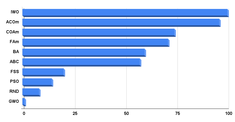
Fig. 4. Histogram of the final results of testing algorithms

Conclusions on the properties of the Invasive Weed Optimization (IWO) algorithm:

Pros:
1. High speed.
2. The algorithm works well with various types of functions, both smooth and discrete.
3. Good scalability.

Cons:
1. Numerous parameters (although they are self-explanatory).