Population optimization algorithms: Firefly Algorithm (FA)

Contents

1. Introduction
2. Algorithm description
3. Test results

1. Introduction

Nature has always been an inspiration for many metaheuristic algorithms. It managed to find solutions to problems without prompting, based on individual experience. Natural selection and survival of the fittest were the main motivation for the creation of early metaheuristic algorithms. In nature, animals communicate with each other in many ways. Fireflies use their ability to blink to communicate. There are about 2000 species of fireflies with their own special flash patterns. They usually produce a short flash with a specific pattern. The light and its intensity become the result of biochemical processes called bioluminescence. It is believed that the main function of such flashes is to attract mating patterns and potential victims. Some tropical fireflies can synchronize their flashes, thus demonstrating an example of biological self-organization. The intensity of light, as a function of distance from its source, obeys an inverse square law, so the flickering light coming from a firefly causes fireflies around it to react within sight of the flash.

There are two variants of population optimization algorithms inspired by the behavior of fireflies: the Firefly Algorithm and the Glowworm Swarm Optimization (GSO) algorithm. The main difference between firefly and glowworms is that the latter are wingless. In this article, we will consider the first type of the optimization algorithm.

2. Algorithm description

The firefly algorithm (F-algorithm) was proposed by X-Sh. Yang at the University of Cambridge (UK) in 2007 and immediately attracted the attention of optimization researchers. The firefly algorithm is part of a family of swarm intelligence algorithms that have recently shown impressive results in solving optimization problems. The firefly algorithm, in particular, is used to solve continuous and discrete optimization problems.

The firefly algorithm has three rules based on the flickering characteristics of real fireflies. The rules are as follows:

1. All fireflies will move towards more attractive and bright counterparts.
2. The degree of attraction of a firefly is proportional to its brightness, which decreases as the distance from another firefly increases due to the fact that the air absorbs light. Therefore, between any two flickering fireflies, the less bright one will move towards the brighter one. If there is no brighter or more attractive counterpart, a firefly will move randomly.
3. The brightness or light intensity of the firefly is determined by the value of the objective function of the problem.

Initially, at the beginning of the algorithm, all fireflies are randomly dispersed throughout the search space. The algorithm then determines the optimal partitions based on two phases:

1. Change in light intensity - the brightness of the firefly in its current position is reflected in the value of its fitness, moving towards an attractive firefly.
2. The firefly changes its position by observing the light intensity of neighboring fireflies.

Now we can dive into the intricacies of firefly optimization in more detail. The essence of the algorithm is clearly shown in Figure 1.

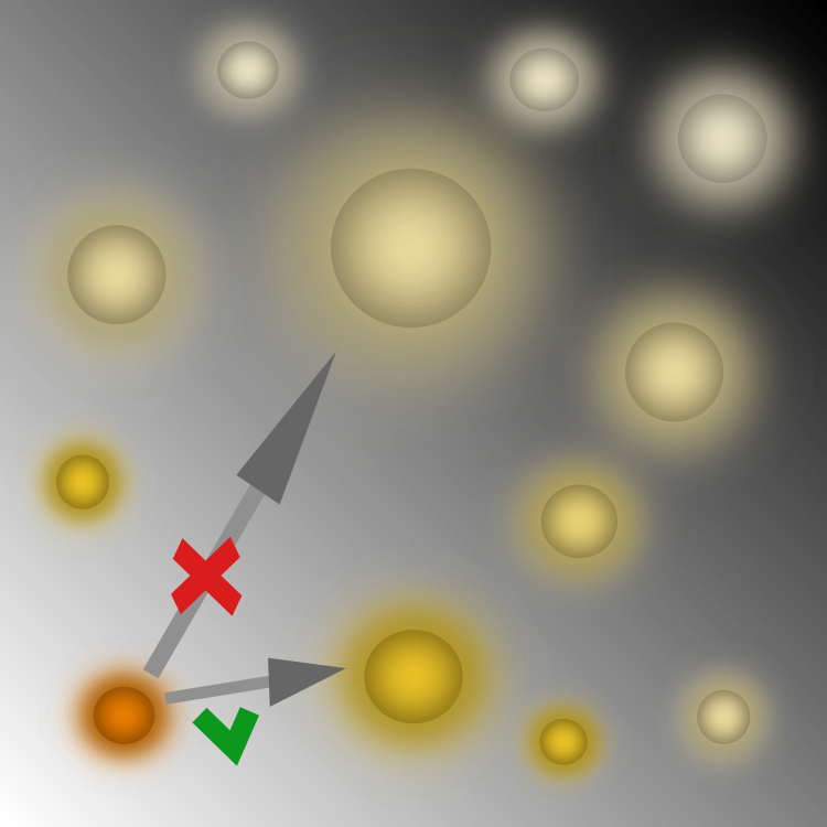
Fig. 1. Fireflies in the search space. Visibility decreases with increasing distance

The main idea behind the search principle is a non-linear decrease in visibility with increasing distance between fireflies. Without this non-linear relationship, each firefly would move deterministically towards a brighter light source. However, as we see in Figure 1, the firefly does not choose its brightest relative, since its light is less noticeable due to the absorption of light by the environment. Instead, it chooses a less bright counterpart (albeit the brightest in its environment). This feature explains the good ability of the algorithm to divide into smaller swarms. This occurs naturally only due to the non-linear function of light absorption from distance. In Figure 2 below, we can see the function of visibility versus distance for the algorithm with different values of the absorption coefficient of the gamma medium, which is one of the algorithm parameters.

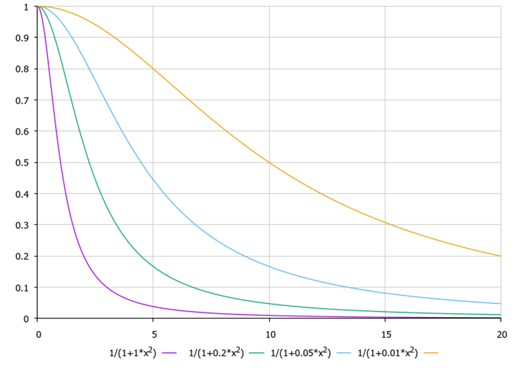
Fig. 2. The function of the transparency of the medium from the distance f(x), where the gamma transparency coefficient is equal to 1.0, 0.2, 0.05, 0.01, respectively.

When gamma tends to infinity, the environment becomes opaque, and when gamma is zero, the environment is completely transparent, and each firefly sees the other at any distance in the search space. What happens if gamma = 0.0? All fireflies will fly to the brightest relative converging to some non-optimal point. So, the algorithm will not converge remaining stuck in one of the local extrema. What happens if the environment is completely opaque? The fireflies will not see anyone more attractive than themselves. According to the concept proposed by the author of the algorithm, not seeing anyone better than oneself, makes a firefly move randomly. The algorithm will degenerate into a random search. In our rating table of algorithm classification, the random search algorithm takes the last place.  

Let's delve into the further analysis of the algorithm and consider the equations that describe the movements of fireflies. The function of visibility versus distance underlies the calculation of the so-called attractiveness index:

attractiveness = fireflies [k].f / (1.0 + gamma * distance * distance);

where:
attractiveness - self-explanatory
gamma - environment opacity coefficient
distance - Euclidean distance between fireflies
fireflies [k].f - light intensity of k-th firefly

The equation makes it clear that the attractiveness function depends directly on the dimension of the problem and the limits of the distance value, so the author of the algorithm recommends selecting the transparency coefficient for a specific optimization problem. I think that it is inconvenient and time-consuming to do so without knowing in advance how the algorithm will behave, so I think it is necessary to normalize the distance values in the range from 0 to 20. To achieve this, apply the Scale () function we have repeatedly used in other algorithms. The conversion of 'distance' before the attractiveness calculation looks like this:

distance = Scale (distance, 0.0, maxDist, 0.0, 20.0, false);

where:

maxDist - maximum Euclidean distance between a pair of fireflies among all others

In this case, the attractiveness of fireflies will not depend on the dimension of the problem and there is no need to select the gamma coefficient for a specific optimization problem. The attractiveness function determines what kind of mate choice each firefly will make. This choice is strictly determined. The influence of the attractiveness of fireflies to each other determines the beta coefficient (the second parameter of the algorithm). How are the search capabilities of the algorithm ensured if the choice of fireflies is already determined in advance at each corresponding iteration? To achieve this, a random vector component and the third algorithm parameter (alpha) are introduced. The complex behavioral relationships of fireflies would look like this:

fireflies [i].c [c] = Xj + beta * (Xi - Xj) + alpha * r * v [c];

where:
fireflies [i].c [c] - c-th coordinate of the i-th firefly
beta - fireflies attraction influence coefficient
alpha - coefficient that affects the random component when moving fireflies, giving deviations from the movement target
r - random number in the range [-1.0;1.0]
v[c] - vector component characterizing the distance between the extreme points of the search range by the c-th coordinate
Хj - corresponding coordinate of the firefly in the pair, to which there will be movement
Xi - corresponding coordinate of the firefly the movement is calculated for

Now it is time to describe the algorithm code. It is relatively simple. Let's consider it in more detail.

A firefly will be described with a simple structure S_Firefly featuring two components, namely [] - coordinates, f - firefly's luminosity (fitness function). Since for each firefly there is only one individual at the corresponding iteration, to which it will move forming a pair, we do not risk overwriting the coordinates when calculating the next movement. For this purpose, I will introduce a special structure considered below.

//——————————————————————————————————————————————————————————————————————————————
struct S_Firefly
{
  double c  []; //coordinates
  double f;     //the value of the fitness function
};
//——————————————————————————————————————————————————————————————————————————————

The S_Attractiveness structure is meant for storing the attractiveness value and the number of the corresponding firefly as a pair. Each firefly does not move towards the coordinates of the most attractive one, but towards the coordinates where its partner has already moved. There is some discrepancy in this with the algorithm version described by the author, but this is how it works better.

//——————————————————————————————————————————————————————————————————————————————
struct S_Attractiveness
{
  double a; //attractiveness
  int    i; //index of the most attractive firefly
};
//——————————————————————————————————————————————————————————————————————————————

The firefly algorithm is described using the C_AO_FA class. There are three public methods here, one of which is Init() for initial initialization and two public methods required to be called at each iteration - Flight() and Luminosity(), private helper methods and members for storing parameter constants.

//——————————————————————————————————————————————————————————————————————————————
class C_AO_FA
{
  //----------------------------------------------------------------------------
  public: S_Firefly fireflies []; //fireflies
  public: double    rangeMax  []; //maximum search range
  public: double    rangeMin  []; //minimum search range
  public: double    rangeStep []; //step search
  public: double    cB        []; //best coordinates
  public: double    fB;           //FF of the best coordinates

  public: void Init (const int    paramsP,  //number of opt. parameters
                     const int    sizeP,    //swarm size
                     const double alphaP,   //alpha, randomness in motion
                     const double betaP,    //beta, effect of attractiveness
                     const double gammaP);  //gamma, transparency of the environment

  public: void Flight ();
  public: void Luminosity ();

  //----------------------------------------------------------------------------
  private: S_Attractiveness att [];
  private: int    swarmSize;
  private: int    params;
  private: double maxDist;
  private: double v [];

  private: double alpha;      //randomness in motion
  private: double beta;       //effect of attractiveness
  private: double gamma;      //transparency of the environment
  private: bool   luminosity;

  private: double SeInDiSp  (double In, double inMin, double inMax, double step);
  private: double RNDfromCI (double min, double max);
  protected: double Scale   (double In, double InMIN, double InMAX, double OutMIN, double OutMAX,  bool revers);
};
//——————————————————————————————————————————————————————————————————————————————

The Init() open method is used for initialization and should be called before the start of each optimization. Its parameters are superstructure parameters for the algorithm. The method will allocate memory for arrays and reset the luminosity value of the global and each individual firefly.

//——————————————————————————————————————————————————————————————————————————————
void C_AO_FA::Init (const int    paramsP, //number of opt. parameters
                    const int    sizeP,   //swarm size
                    const double alphaP,  //alpha, randomness in motion
                    const double betaP,   //beta, effect of attractiveness
                    const double gammaP)  //gamma, transparency of the environment
{
  fB = -DBL_MAX;

  params    = paramsP;
  swarmSize = sizeP;
  alpha     = alphaP;
  beta      = betaP;
  gamma     = gammaP;

  ArrayResize (rangeMax,  params);
  ArrayResize (rangeMin,  params);
  ArrayResize (rangeStep, params);
  ArrayResize (v,         params);
  ArrayResize (att,       swarmSize);

  luminosity = false;

  ArrayResize (fireflies, swarmSize);

  for (int i = 0; i < swarmSize; i++)
  {
    ArrayResize (fireflies [i].c,  params);
    fireflies [i].f = -DBL_MAX;
  }

  ArrayResize (cB, params);
}
//——————————————————————————————————————————————————————————————————————————————

Consider the first public method called on each iteration - Flight(). The main logic of the algorithm is concentrated in this method, so it is necessary to consider it in more detail. The 'luminosity' variable serves as a flag allowing us to determine whether the algorithm is running on the first iteration or on subsequent ones. If the flag is not set, it is necessary to distribute the fireflies randomly in the coordinate space in accordance with the uniform distribution. Along with this action, we set the displacement vector for each coordinate and immediately calculate the maximum possible Euclidean distance that can be between fireflies (as already mentioned, this is necessary to normalize the distances between fireflies in order to avoid the dependence of the environment transparency coefficient on the dimension of the problem). After these operations, enable the 'luminosity' flag.

if (!luminosity)
{
  fB = -DBL_MAX;

  //--------------------------------------------------------------------------
  double summCoordinates = 0.0;
  for (int c = 0; c < params; c++)
  {
    v [c] = rangeMax [c] - rangeMin [c];
    summCoordinates += pow (v [c], 2.0);
  }
  maxDist = pow (summCoordinates, 0.5);

  //--------------------------------------------------------------------------
  for (int s = 0; s < swarmSize; s++)
  {
    for (int k = 0; k < params; k++)
    {
      fireflies [s].c  [k] = RNDfromCI (rangeMin [k], rangeMax [k]);
      fireflies [s].c  [k] = SeInDiSp (fireflies [s].c [k], rangeMin [k], rangeMax [k], rangeStep [k]);
    }
  }

  luminosity = true;
}

From the second and further iterations, after the fireflies were randomly distributed at the first iteration and began to glow (the fitness function was calculated for them), it is possible to calculate the degree of attractiveness for each firefly. To do this, we need to calculate the Euclidean distance between all possible pairs of fireflies. To do this, simply add the squares of the differences in coordinates, and find the root from their sum. The calculated distance will be used in the attractiveness calculation equation. This is how we get the only possible pair for each firefly. Determine the maximum luminosity among all fireflies. This will be required in order to determine the brightest firefly, for which it will not be possible to find a pair and which will wander in space alone. Well, perhaps, it will be more lucky during the next iteration.

//measure the distance between all------------------------------------------
for (int i = 0; i < swarmSize; i++)
{
  att [i].a = -DBL_MAX;

  for (int k = 0; k < swarmSize; k++)
  {
    if (i == k) continue;

    summCoordinates = 0.0;
    for (int c = 0; c < params; c++) summCoordinates += pow (fireflies [i].c [c] - fireflies [k].c [c], 2.0);

    distance = pow (summCoordinates, 0.5);
    distance = Scale (distance, 0.0, maxDist, 0.0, 20.0, false);
    attractiveness = fireflies [k].f / (1.0 + gamma * distance * distance);

    if (attractiveness > att [i].a)
    {
      att [i].a = attractiveness;
      att [i].i = k;
    }

    if (fireflies [i].f > maxF) maxF = fireflies [i].f;
  }
}

This part of the Flight() method code is responsible for the flight of the fireflies. For the unfortunate firefly, whose luminosity is greater than all the others, the calculation is performed somewhat differently. We add the movement vector to its current position through the alpha coefficient multiplied by a random number [-1.0;1.0]. Theoretically, in the algorithm, this acts as an additional study of the best solution with the expectation that it will be even better, however, as we will see later, this technique will turn out to be useless. At this stage, we consider the classical version of the algorithm.

For all other fireflies, for which a pair has already been found, the calculation of the movement will consist in moving towards the appropriate pair with the addition of a random component (I mentioned it earlier).

//flight--------------------------------------------------------------------
for (int i = 0; i < swarmSize; i++)
{
  if (fireflies [i].f >= maxF)
  {
    for (int c = 0; c < params; c++)
    {
      r  = RNDfromCI (-1.0, 1.0);
      fireflies [i].c [c] = fireflies [i].c [c] + alpha * r * v [c];
      fireflies [i].c [c] = SeInDiSp (fireflies [i].c [c], rangeMin [c], rangeMax [c], rangeStep [c]); 
    }
  }
  else
  {
    for (int c = 0; c < params; c++)
    {
      r  = RNDfromCI (-1.0, 1.0);
      Xi = fireflies [i].c [c];
      Xj = fireflies [att [i].i].c [c];
      fireflies [i].c [c] = Xj + beta * (Xi - Xj) + alpha * r * v [c];
      fireflies [i].c [c] = SeInDiSp (fireflies [i].c [c], rangeMin [c], rangeMax [c], rangeStep [c]);
    }
  }
}

A simple open method called on every iteration. Here we will update the best solution.

//——————————————————————————————————————————————————————————————————————————————
void C_AO_FA::Luminosity ()
{
  for (int i = 0; i < swarmSize; i++)
  {
    if (fireflies [i].f > fB)
    {
      fB = fireflies [i].f;
      ArrayCopy (cB, fireflies [i].c, 0, 0, WHOLE_ARRAY);
    }
  }
}
//——————————————————————————————————————————————————————————————————————————————

Let's move on to the tests. Let's look at the results of the algorithm on the test functions:

2022.12.16 13:39:00.102    Test_AO_FA (EURUSD,M1)    =============================
2022.12.16 13:39:05.930    Test_AO_FA (EURUSD,M1)    1 Skin's; Func runs 10000 result: 4.901742065217812
2022.12.16 13:39:05.930    Test_AO_FA (EURUSD,M1)    Score: 0.99603
2022.12.16 13:39:13.579    Test_AO_FA (EURUSD,M1)    20 Skin's; Func runs 10000 result: 3.2208359936020665
2022.12.16 13:39:13.579    Test_AO_FA (EURUSD,M1)    Score: 0.59468
2022.12.16 13:39:53.607    Test_AO_FA (EURUSD,M1)    500 Skin's; Func runs 10000 result: 0.98491319842575
2022.12.16 13:39:53.607    Test_AO_FA (EURUSD,M1)    Score: 0.06082
2022.12.16 13:39:53.607    Test_AO_FA (EURUSD,M1)    =============================
2022.12.16 13:39:59.313    Test_AO_FA (EURUSD,M1)    1 Forest's; Func runs 10000 result: 1.578196881663454
2022.12.16 13:39:59.313    Test_AO_FA (EURUSD,M1)    Score: 0.89271
2022.12.16 13:40:07.274    Test_AO_FA (EURUSD,M1)    20 Forest's; Func runs 10000 result: 0.3101994341994826
2022.12.16 13:40:07.274    Test_AO_FA (EURUSD,M1)    Score: 0.17546
2022.12.16 13:40:49.159    Test_AO_FA (EURUSD,M1)    500 Forest's; Func runs 10000 result: 0.06829102669136165
2022.12.16 13:40:49.159    Test_AO_FA (EURUSD,M1)    Score: 0.03863
2022.12.16 13:40:49.159    Test_AO_FA (EURUSD,M1)    =============================
2022.12.16 13:40:54.895    Test_AO_FA (EURUSD,M1)    1 Megacity's; Func runs 10000 result: 8.2
2022.12.16 13:40:54.895    Test_AO_FA (EURUSD,M1)    Score: 0.68333
2022.12.16 13:41:02.777    Test_AO_FA (EURUSD,M1)    20 Megacity's; Func runs 10000 result: 1.5900000000000003
2022.12.16 13:41:02.777    Test_AO_FA (EURUSD,M1)    Score: 0.13250
2022.12.16 13:41:43.901    Test_AO_FA (EURUSD,M1)    500 Megacity's; Func runs 10000 result: 0.2892
2022.12.16 13:41:43.901    Test_AO_FA (EURUSD,M1)    Score: 0.02410
2022.12.16 13:41:43.901    Test_AO_FA (EURUSD,M1)    =============================
2022.12.16 13:41:43.901    Test_AO_FA (EURUSD,M1)    All score for C_AO_FA: 0.39980648892951776

The results are unimpressive, to put it mildly. The algorithm is only slightly better than PSO, FSS, GWO in individual tests. However, in the total rating indicator, it is in the second position from the bottom leaving only the random search algorithm behind. Considering all this, the idea arose to revise the calculation of estimated indicators in tests. In the following articles, I will switch to a more convenient rating calculation scheme, while in the current article, I will add the histogram of the final results. It will clearly show the performance ratio between individual algorithms.

The classic Firefly algorithm is easy to implement. However, studies show that it converges slowly and easily falls into the local extremum trap for multimodal problems. In addition, it lacks coefficients that are parametrically dependent on the current iteration. Hence, one of the objectives of the study was modifying the standard Firefly algorithm to improve its performance.

The very idea of the algorithm is quite original and it would be a pity to leave everything as it is and not try to improve its characteristics. Therefore, I attempted to modify the algorithm by replacing the random component with a Levy flight. Levy's flight cannot improve the search ability for every algorithm. After considering the cuckoo search algorithm, I tried to improve other algorithms using this method, but this did not bring the expected results. Apparently, this should be consistent in some way with the internal search strategy within the algorithm complementing it. In this particular case, the application of Levy's Flight gave a striking effect - the capabilities of the algorithm increased dramatically. We will talk about this in the part of the article about the test results.

Here is the part of the code where the change was made. First, in the classic version, the firefly with the best luminosity moves in a random direction from its current position. Then our best firefly moves from the best global position trying to improve not its current position, but the solution as a whole. Add a random number of the Levy's flight distribution (distribution with heavy tails) with the same alpha coefficient, taking into account the movement vector, to the coordinates of the best solution. This really made it possible to improve the coordinates of the global solution by refining the neighboring area.

As you can see, the behavior of the rest of the fireflies now obeys the same classical rules, albeit adjusted for the random component of Levy's flight. That is the whole modification made to the algorithm.

//flight--------------------------------------------------------------------
for (int i = 0; i < swarmSize; i++)
{
  if (fireflies [i].f >= maxF)
  {
    for (int c = 0; c < params; c++)
    {
      r1 = RNDfromCI (0.0, 1.0);
      r1 = r1 > 0.5 ? 1.0 : -1.0;
      r2 = RNDfromCI (1.0, 20.0);

      fireflies [i].c [c] = cB [c] + alpha * r1 * pow (r2, -2.0) * v [c];
      fireflies [i].c [c] = SeInDiSp (fireflies [i].c [c], rangeMin [c], rangeMax [c], rangeStep [c]);
    }
  }
  else
  {
    for (int c = 0; c < params; c++)
    {
      r1 = RNDfromCI (0.0, 1.0);
      r1 = r1 > 0.5 ? 1.0 : -1.0;
      r2 = RNDfromCI (1.0, 20.0);

      Xi = fireflies [i].c [c];
      Xj = fireflies [att [i].i].c [c];

      fireflies [i].c [c] = Xj + beta * (Xi - Xj) + alpha * r1 * pow (r2, -2.0) * v [c];
      fireflies [i].c [c] = SeInDiSp (fireflies [i].c [c], rangeMin [c], rangeMax [c], rangeStep [c]);
    }
  }
}

Levy's flight function chart in Fig. 3. How can the exponent in the function equation affect the behavior of the algorithm? According to my research, as the degree increases, the number of long (heavy tails) jumps decreases relative to short ones, while the algorithm ability to refine coordinates in the vicinity of the best solution improves. Due to the fact that there are few long jumps, the probability of getting stuck in local extrema increases. This effect will be more noticeable when studying discrete functions, while it will not be so pronounced on smooth ones. On the contrary, with a decrease in the exponent, the number of long jumps increases, the search capabilities of the algorithm improve, but the convergence accuracy worsens, so we need the middle ground between accuracy and search. Besides, it can be different depending on the optimization problem.

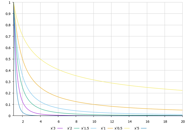
Fig. 3. Levy's flight function, degrees 0.5...3.0 

So, let's move on to the results of the modified version of the algorithm on the test stand. Below you can see how much the performance of the original version has improved compared to the classic one.

2022.12.16 13:07:15.925    Test_AO_FAm (EURUSD,M1)    =============================
2022.12.16 13:07:21.544    Test_AO_FAm (EURUSD,M1)    1 Skin's; Func runs 10000 result: 4.854437214435259
2022.12.16 13:07:21.544    Test_AO_FAm (EURUSD,M1)    Score: 0.98473
2022.12.16 13:07:29.518    Test_AO_FAm (EURUSD,M1)    20 Skin's; Func runs 10000 result: 4.588539001298423
2022.12.16 13:07:29.518    Test_AO_FAm (EURUSD,M1)    Score: 0.92124
2022.12.16 13:08:12.587    Test_AO_FAm (EURUSD,M1)    500 Skin's; Func runs 10000 result: 1.981278990090829
2022.12.16 13:08:12.587    Test_AO_FAm (EURUSD,M1)    Score: 0.29872
2022.12.16 13:08:12.587    Test_AO_FAm (EURUSD,M1)    =============================
2022.12.16 13:08:18.336    Test_AO_FAm (EURUSD,M1)    1 Forest's; Func runs 10000 result: 1.7665409595127233
2022.12.16 13:08:18.336    Test_AO_FAm (EURUSD,M1)    Score: 0.99924
2022.12.16 13:08:26.432    Test_AO_FAm (EURUSD,M1)    20 Forest's; Func runs 10000 result: 0.6261364994589462
2022.12.16 13:08:26.432    Test_AO_FAm (EURUSD,M1)    Score: 0.35417
2022.12.16 13:09:10.587    Test_AO_FAm (EURUSD,M1)    500 Forest's; Func runs 10000 result: 0.14269062630878
2022.12.16 13:09:10.587    Test_AO_FAm (EURUSD,M1)    Score: 0.08071
2022.12.16 13:09:10.587    Test_AO_FAm (EURUSD,M1)    =============================
2022.12.16 13:09:16.393    Test_AO_FAm (EURUSD,M1)    1 Megacity's; Func runs 10000 result: 10.0
2022.12.16 13:09:16.393    Test_AO_FAm (EURUSD,M1)    Score: 0.83333
2022.12.16 13:09:24.373    Test_AO_FAm (EURUSD,M1)    20 Megacity's; Func runs 10000 result: 1.7899999999999998
2022.12.16 13:09:24.373    Test_AO_FAm (EURUSD,M1)    Score: 0.14917
2022.12.16 13:10:09.298    Test_AO_FAm (EURUSD,M1)    500 Megacity's; Func runs 10000 result: 0.5076
2022.12.16 13:10:09.298    Test_AO_FAm (EURUSD,M1)    Score: 0.04230
2022.12.16 13:10:09.298    Test_AO_FAm (EURUSD,M1)    =============================
2022.12.16 13:10:09.298    Test_AO_FAm (EURUSD,M1)    All score for C_AO_FAm: 0.5181804234713119

As you can see, the modified algorithm not only shows better results but takes a leading position in the rating table. Let's take a closer look at the results in the next section. Below is an animation of the modified version of the algorithm on the test stand.

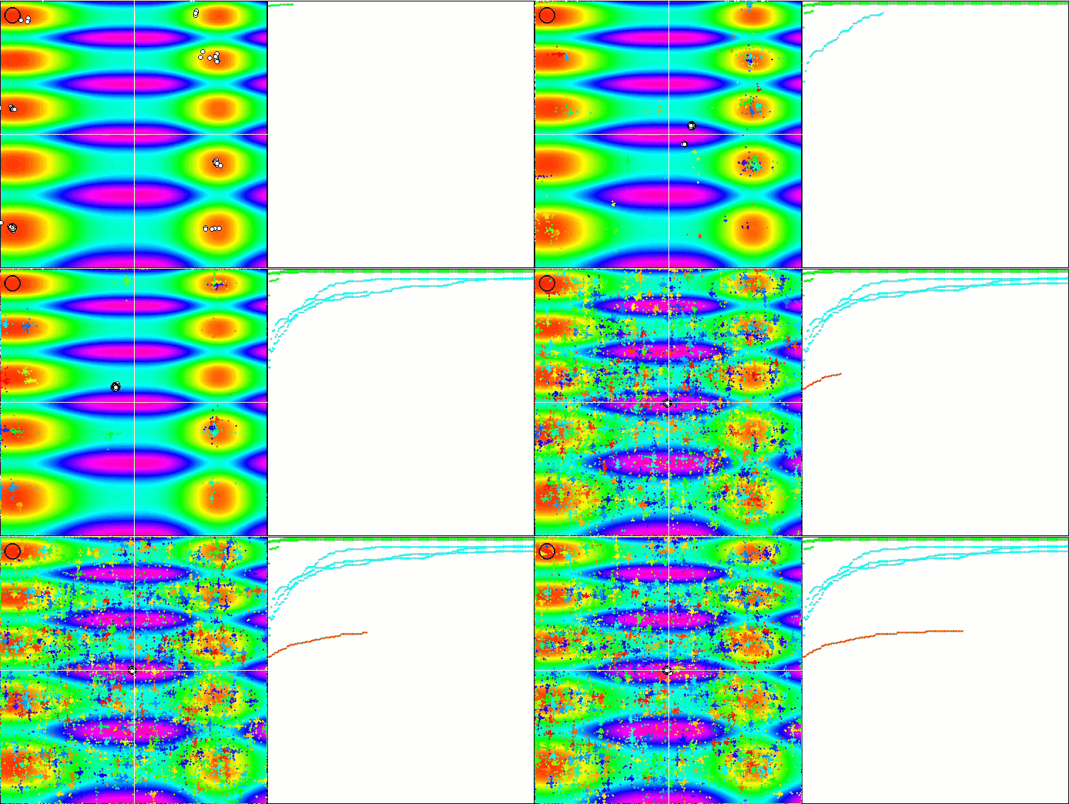
  FAm on the Skin test function.

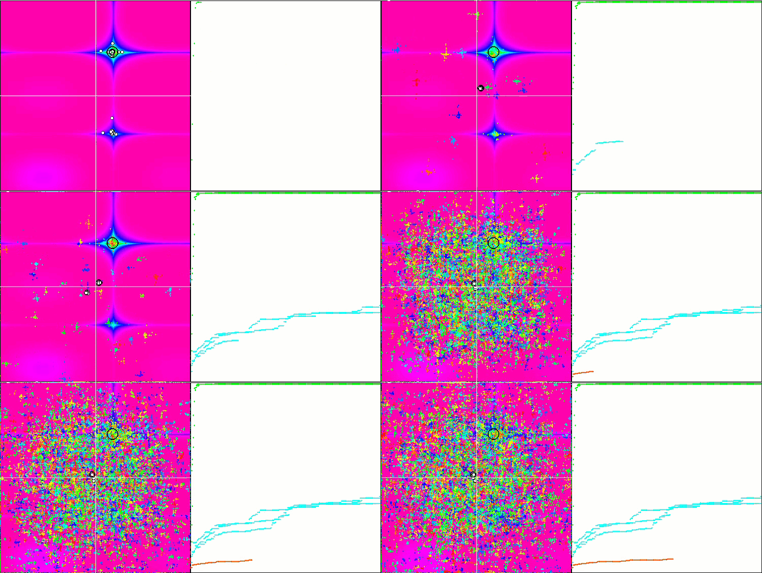
  FAm on the Forest test function.

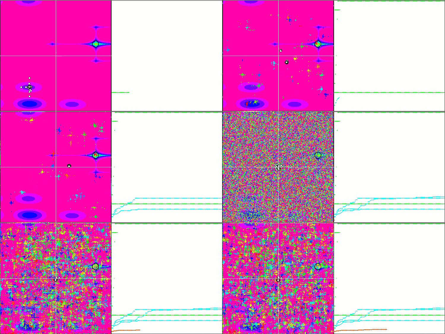
  FAm on the Megacity test function.

3. Test results

The modified firefly algorithm (FAm) performed excellently in all the tests. Generally, the results depend on the settings of the algorithm. In case of some settings, 100% convergence was achieved on all three functions with two variables. The high scalability of the algorithm provides leadership in tests with 40 and 1000 parameters. The beta and gamma parameters have a strong influence making it possible to obtain both high convergence and resistance to getting stuck in local extrema. The results vary widely, which in general can be attributed to the disadvantages of the algorithm. With all else being equal, the algorithm is the strongest among those considered earlier. It can be recommended for use in a very wide range of tasks, including machine learning and artificial intelligence tasks, in particular when training neural networks.

Below is the final rating table, in which the modified firefly algorithm takes the lead. Unfortunately, the classical algorithm, despite its originality, could not achieve good results. The selection of tuning parameters did not bring success either.

AO	Description	Skin			Skin final	Forest			Forest final	Megacity (discrete)			Megacity final	Final result
		2 params (1 F)	40 params (20 F)	1000 params (500 F)		2 params (1 F)	40 params (20 F)	1000 params (500 F)		2 params (1 F)	40 params (20 F)	1000 params (500 F)
FAm	firefly algorithm M	0.98473	0.92124	0.29872	0.73490	0.99924	0.35417	0.08071	0.47804	0.83333	0.14917	0.04230	0.34160	0.51817889
COAm	cuckoo optimization algorithm M	1.00000	0.85911	0.14316	0.66742	0.99283	0.28787	0.04551	0.44207	1.00000	0.24917	0.03537	0.42818	0.51255778
ACOm	ant colony optimization M	0.98229	0.79108	0.12602	0.63313	1.00000	0.62077	0.11521	0.57866	0.38333	0.44000	0.02377	0.28237	0.49805222
ABCm	artificial bee colony M	1.00000	0.63922	0.08076	0.57333	0.99908	0.20112	0.03785	0.41268	1.00000	0.16333	0.02823	0.39719	0.46106556
ABC	artificial bee colony	0.99339	0.73381	0.11118	0.61279	0.99934	0.21437	0.04215	0.41862	0.85000	0.16833	0.03130	0.34988	0.46043000
GWO	grey wolf optimizer	0.99900	0.48033	0.18924	0.55619	0.83844	0.08755	0.02555	0.31718	1.00000	0.10000	0.02187	0.37396	0.41577556
FSS	fish school search	0.99391	0.5692	0.11341	0.55884	0.85172	0.12143	0.03223	0.33513	0.91667	0.08583	0.02583	0.34278	0.41224778
PSO	particle swarm optimisation	0.99627	0.38080	0.05089	0.47599	0.93772	0.14540	0.04856	0.37723	1.00000	0.09333	0.02233	0.37189	0.40836667
FA	firefly algorithm	0.99603	0.59468	0.06082	0.55051	0.89271	0.17546	0.03863	0.36893	0.68333	0.13250	0.02410	0.27998	0.39980649
RND	random	0.99932	0.44276	0.06827	0.50345	0.83126	0.11524	0.03048	0.32566	0.83333	0.09000	0.02403	0.31579	0.38163222

Starting from this article, I will publish a histogram, on which the best algorithm at the time of testing will have 100 conditional points, while the worst one will have 1 point. I think, this is the most convenient display method in terms of visual perception since we can clearly see the scale of the final results of the rating table algorithms. Now we can see how much the random algorithm lags behind the leader.

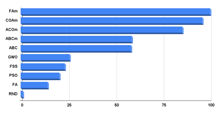
Fig. 4. Histogram of the final results of testing algorithms

As you might remember, metaheuristic algorithms are approximate methods for solving optimization problems that use the property of randomness with a reasonable assumption in their search engine and try to improve the quality of the available solutions through iterations from a randomly generated set of valid solutions by examining and using the solution space. Although these algorithms are not guaranteed to be optimal, they are tested to give a reasonable and acceptable solution. In addition, they have the advantage in the fact that the behavior of the problem does not greatly affect them, and this is what makes them useful in many tasks. The presence of many available algorithms makes it possible to choose the appropriate one for solving a problem, depending on its behavior.

Since the advent of evolutionary algorithms, there has been a lot of research into heuristic algorithms. Implementation of new algorithms has been one of the leading research areas. Currently, there are more than 40 metaheuristic algorithms. Most of them are created by simulating scenarios from nature.

The pros and cons refer to a modified version of the Firefly Algorithm (FAm).

Pros:

• Simple implementation. Easy to modify.
• High scalability.
• High convergence (may vary depending on algorithm settings).
• The ability to cluster the region of the search space into separate groups around local extrema.

Cons:

• Strong influence of settings on optimization results.
• With some settings, the algorithm is prone to getting stuck in local extrema.

Each article features an archive that contains updated current versions of the algorithm codes for all previous articles. Each new article is the accumulated personal experience of the author and the conclusions and judgments are based on the experiments carried out on a special test stand developed for this purpose.