予測による統計的裁定取引

はじめに

統計的裁定取引とは、数理モデルを活用して、関連する金融商品間の価格の非効率性を利用する高度な金融戦略です。通常、株式、債券、デリバティブに適用されるこのアプローチは、相関関係、相関、ピアソン係数について深い理解を必要とします。これは、市場機会を特定し、活用するための重要なツールです。

金融における相関は、2つの証券が互いに関連してどの程度密接に動くかを測定し、関連性の程度を数値化します。正の相関は、証券が通常同じ方向に動くことを示し、負の相関は、それらが逆方向に動くことを意味します。トレーダーはこれらの関係を分析し、将来の値動きを予測します。

より微妙な統計的性質である共和分は、2つ以上の時系列変数の線形結合が時間と共に安定しているかどうかを調べるもので、相関関係を超えるものです。もっと簡単に言えば、個々の証券は異なる経路をたどるかもしれませんが、その相対的な動きはある均衡によって結ばれており、その均衡に回帰する傾向があります。この概念はペア取引において極めて重要であり、その目的は、価格が履歴的に一緒に動き、今後もそうなると予想される銘柄のペアを特定することです。

ピアソン係数は、2つの変数の間の線形関係の強さと方向を計算する統計的尺度です。ピアソン係数の値の範囲は-1から1までで、1は完全な正の線形関係、-1は完全な負の線形関係、0は線形関係なしを意味します。統計的裁定取引では、2つの資産間のピアソン係数の絶対値が高ければ、長期的な平均関係に戻ると仮定して、潜在的な取引機会を示唆する可能性があります。

統計的裁定取引戦略を実施するトレーダーは、アルゴリズムと高頻度取引システムを利用して取引を監視し、執行しています。これらのシステムは、膨大な量のデータを処理し、資産価格関係の異常を迅速に検出することができます。この戦略では、相関性のある資産の価格が過去の平均に収束すると想定しており、トレーダーは価格調整で利益を上げることができます。

しかし、統計的裁定取引の成功は、洗練された数学的モデルだけでなく、データを解釈し、変化する市場状況に基づいて戦略を調整するトレーダーの能力にも依存します。急激な経済変動、市場心理、政治的な出来事などの要因は、最も安定した関係をも混乱させ、より高いレベルのリスクをもたらす可能性があります。

簡単な例による説明

相関関係は、2つのものがどのように関連しているかを測るものです。あなたと親友が土曜日にいつも一緒に映画を観に行くとします。これは相関関係の例です。あなたが映画館に行くと、あなたの友人もそこにいます。正の相関関係は、一方が上昇すれば他方も上昇することを意味します。負の場合は、一方が増加すると他方が減少します。相関がゼロであれば、両者の間には何の関係もありません。

共和分とは、2つ以上の変数が、短期的には独立して変動していても長期的には何らかの関係を持っているという状況を説明するために使用される統計的概念です。ロープで結ばれた2人のスイマーを想像してください。2人はプールで自由に泳ぐことができますが、互いに遠くへ移動することはできません。共和分は、一時的な差異にもかかわらず、これらの変数が常に共通の長期的均衡またはトレンドに戻ることを示します。

ピアソン係数は、2つの変数がどの程度線形に関連しているかを測定します。係数が+1に近い場合は、一方の変数が増加すると他方の変数も増加するという直接的な依存関係を示しています。係数が-1に近いということは、一方が増加すると他方が減少することを意味し、逆の関係を示しています。0は線形のつながりがないことを意味します。例えば、気温と冷たい飲み物の販売数を測定することで、ピアソン係数を用いてこれらの要因がどのように関連しているかを理解することができます。

まとめると、統計的裁定取引は、経済学、金融学、数学の要素を組み合わせた複雑ですが、利益を生む可能性のある取引戦略です。高度な統計概念を理解するだけでなく、市場分析と執行のための高速アルゴリズムを導入する能力も必要とされます。

計算

どのペアが共和分で相関しているかを知るには、以下の.pyを使用することができます。

import MetaTrader5 as mt5
import pandas as pd
from scipy.stats import pearsonr
from statsmodels.tsa.stattools import coint
import numpy as np

# Conectar con MetaTrader 5
if not mt5.initialize():
    print("No se pudo inicializar MT5")
    mt5.shutdown()

# Obtener la lista de símbolos
symbols = mt5.symbols_get()
symbols = [s.name for s in symbols if s.name.startswith('EUR') or s.name.startswith('USD') or s.name.endswith('USD')]  # Filtrar símbolos por ejemplo

# Descargar datos históricos y almacenar en un diccionario
data = {}
for symbol in symbols:
    rates = mt5.copy_rates_from_pos(symbol, mt5.TIMEFRAME_D1, 0, 365)  # Último año, diario
    if rates is not None:
        df = pd.DataFrame(rates)
        df['time'] = pd.to_datetime(df['time'], unit='s')
        data[symbol] = df.set_index('time')['close']

# Cerrar la conexión con MT5
mt5.shutdown()

# Calcular el coeficiente de Pearson y probar la cointegración para cada par de símbolos
cointegrated_pairs = []
for i in range(len(symbols)):
    for j in range(i + 1, len(symbols)):
        if symbols[i] in data and symbols[j] in data:
            common_index = data[symbols[i]].index.intersection(data[symbols[j]].index)
            if len(common_index) > 30:  # Asegurarse de que hay suficientes puntos de datos
                corr, _ = pearsonr(data[symbols[i]][common_index], data[symbols[j]][common_index])
                if abs(corr) > 0.8:  # Correlación fuerte
                    score, p_value, _ = coint(data[symbols[i]][common_index], data[symbols[j]][common_index])
                    if p_value < 0.05:  # P-valor menor que 0.05
                        cointegrated_pairs.append((symbols[i], symbols[j], corr, p_value))

# Filtrar y mostrar solo los pares cointegrados con p-valor menor de 0.05
print(f'Total de pares con fuerte correlación y cointegrados: {len(cointegrated_pairs)}')
for sym1, sym2, corr, p_val in cointegrated_pairs:
    print(f'{sym1} - {sym2}: Correlación={corr:.4f}, P-valor de Cointegración={p_val:.4f}')

その結果、このようになりました。

Total de pares con fuerte correlación y cointegrados: 54
EURUSD - USDBGN: Correlación=-0.9957, P-valor de Cointegración=0.0000
EURUSD - USDHRK: Correlación=-0.9972, P-valor de Cointegración=0.0000
GBPUSD - USDPLN: Correlación=-0.8633, P-valor de Cointegración=0.0406
GBPUSD - GBXUSD: Correlación=0.9998, P-valor de Cointegración=0.0000
GBPUSD - EURSGD: Correlación=0.8061, P-valor de Cointegración=0.0191
USDCHF - EURCHF: Correlación=0.8324, P-valor de Cointegración=0.0356
USDJPY - EURDKK: Correlación=0.8338, P-valor de Cointegración=0.0200
USDJPY - USDTHB: Correlación=0.9012, P-valor de Cointegración=0.0330
AUDUSD - USDCNH: Correlación=-0.8074, P-valor de Cointegración=0.0390
EURCHF - USDKES: Correlación=-0.9104, P-valor de Cointegración=0.0048
EURJPY - EURRON: Correlación=0.8177, P-valor de Cointegración=0.0333
EURJPY - USDCOP: Correlación=-0.9361, P-valor de Cointegración=0.0125
EURJPY - USDLAK: Correlación=0.9508, P-valor de Cointegración=0.0410
EURJPY - EURDKK: Correlación=0.8525, P-valor de Cointegración=0.0136
EURJPY - EURMXN: Correlación=-0.8785, P-valor de Cointegración=0.0172
EURJPY - USDTRY: Correlación=0.9564, P-valor de Cointegración=0.0102
EURNZD - NZDUSD: Correlación=-0.8505, P-valor de Cointegración=0.0455
EURNZD - EURDKK: Correlación=0.8242, P-valor de Cointegración=0.0017
EURCZK - USDCLP: Correlación=0.9655, P-valor de Cointegración=0.0001
USDCLP - USDCZK: Correlación=0.8972, P-valor de Cointegración=0.0147
USDCLP - USDARS: Correlación=0.8077, P-valor de Cointegración=0.0231
USDCLP - USDIDR: Correlación=0.8569, P-valor de Cointegración=0.0423
USDCLP - USDNGN: Correlación=0.8468, P-valor de Cointegración=0.0436
USDCLP - USDVND: Correlación=0.9021, P-valor de Cointegración=0.0194
USDCZK - USDIDR: Correlación=0.9005, P-valor de Cointegración=0.0086
USDCZK - USDVND: Correlación=0.8306, P-valor de Cointegración=0.0195
USDMXN - USDCOP: Correlación=0.8686, P-valor de Cointegración=0.0286
USDMXN - EURMXN: Correlación=0.9522, P-valor de Cointegración=0.0328
NZDUSD - USDSGD: Correlación=-0.8145, P-valor de Cointegración=0.0097
NZDUSD - USDTHB: Correlación=-0.8094, P-valor de Cointegración=0.0255
ADAUSD - KSMUSD: Correlación=0.9429, P-valor de Cointegración=0.0071
ALGUSD - LNKUSD: Correlación=0.8038, P-valor de Cointegración=0.0454
ATMUSD - MTCUSD: Correlación=0.9423, P-valor de Cointegración=0.0146
BTCUSD - SOLUSD: Correlación=0.9736, P-valor de Cointegración=0.0112
DGEUSD - GLDUSD: Correlación=0.8933, P-valor de Cointegración=0.0136
DGEUSD - USDGHS: Correlación=0.8562, P-valor de Cointegración=0.0101
EOSUSD - UNIUSD: Correlación=0.8176, P-valor de Cointegración=0.0051
ETCUSD - ETHUSD: Correlación=0.9745, P-valor de Cointegración=0.0009
ETCUSD - SOLUSD: Correlación=0.9206, P-valor de Cointegración=0.0093
ETCUSD - UNIUSD: Correlación=0.9236, P-valor de Cointegración=0.0249
ETHUSD - SOLUSD: Correlación=0.9430, P-valor de Cointegración=0.0074
UNIUSD - USDNGN: Correlación=0.8074, P-valor de Cointegración=0.0195
EURNOK - USDNOK: Correlación=0.9065, P-valor de Cointegración=0.0430
EURRON - USDCOP: Correlación=-0.8010, P-valor de Cointegración=0.0097
EURRON - USDCRC: Correlación=-0.8015, P-valor de Cointegración=0.0159
EURRON - USDLAK: Correlación=0.8364, P-valor de Cointegración=0.0349
GBXUSD - EURSGD: Correlación=0.8067, P-valor de Cointegración=0.0180
USDARS - USDVND: Correlación=0.8093, P-valor de Cointegración=0.0268
USDBGN - USDHRK: Correlación=0.9944, P-valor de Cointegración=0.0000
USDCOP - USDTRY: Correlación=-0.9548, P-valor de Cointegración=0.0160
USDCRC - EURDKK: Correlación=-0.8519, P-valor de Cointegración=0.0153
USDHRK - USDDKK: Correlación=0.9954, P-valor de Cointegración=0.0000
USDIDR - USDVND: Correlación=0.8196, P-valor de Cointegración=0.0417
USDSEK - USDSGD: Correlación=0.8346, P-valor de Cointegración=0.0264

すでにフィルタリングされたペアで。

MetaTrader 5でこの値を確認するために、Pearson.mq5指標があります。

//+------------------------------------------------------------------+
//|                                             PearsonIndicator.mq5 |
//|                    Copyright Javier S. Gastón de Iriarte Cabrera |
//|                                       https://www.mql5.com/ja/users/jsgaston/news |
//+------------------------------------------------------------------+
#property copyright "Javier S. Gastón de Iriarte Cabrera"
#property link      "https://www.mql5.com/ja/users/jsgaston/news/"
#property version   "1.00"
#property indicator_separate_window
#property indicator_buffers 1
#property indicator_color1 Red

input string Symbol2 = "GBPUSD";       // Second financial instrument
input int BarsBack = 100;              // Number of bars to include in correlation calculation

double CorrelationBuffer[];

//+------------------------------------------------------------------+
//| Custom indicator initialization function                         |
//+------------------------------------------------------------------+
int OnInit()
  {
   SetIndexBuffer(0, CorrelationBuffer, INDICATOR_DATA);
   PlotIndexSetInteger(0, PLOT_DRAW_TYPE, DRAW_LINE);
   PlotIndexSetString(0, PLOT_LABEL, "Pearson Correlation");
   IndicatorSetString(INDICATOR_SHORTNAME, "Pearson Correlation (" + Symbol() + " & " + Symbol2 + ")");
   return INIT_SUCCEEDED;
  }

//+------------------------------------------------------------------+
//| Custom indicator iteration function                              |
//+------------------------------------------------------------------+
int OnCalculate(const int rates_total,
                const int prev_calculated,
                const datetime &time[],
                const double &open[],
                const double &high[],
                const double &low[],
                const double &close[],
                const long &tick_volume[],
                const long &volume[],
                const int &spread[])
  {
   if (rates_total < BarsBack) return 0; // Ensure enough bars are present

   double prices1[], prices2[];
   ArrayResize(prices1, BarsBack);
   ArrayResize(prices2, BarsBack);

   // Copy historical data for primary symbol
   if (CopyClose(Symbol(), PERIOD_CURRENT, 0, BarsBack, prices1) <= 0)
      {
       Print("Error copying prices for ", Symbol());
       return 0;
      }
   // Copy historical data for secondary symbol
   if (CopyClose(Symbol2, PERIOD_CURRENT, 0, BarsBack, prices2) <= 0)
      {
       Print("Error copying prices for ", Symbol2);
       return 0;
      }

   // Calculate Pearson correlation for the entire buffer
   double correlation = CalculatePearsonCorrelation(prices1, prices2);
   Print("Pearson correlation: ", correlation);

   // Fill the buffer for the indicator
   for (int i = BarsBack; i < rates_total; i++)
     {
      CorrelationBuffer[i] = correlation;  // Update the buffer correctly
     }

   return(rates_total);
  }

//+------------------------------------------------------------------+
//| Calculate Pearson correlation coefficient                        |
//+------------------------------------------------------------------+
double CalculatePearsonCorrelation(double &prices1[], double &prices2[])
  {
   int length = BarsBack;
   double mean1 = 0, mean2 = 0;
   double sum1 = 0, sum2 = 0, sumProd = 0, stdev1 = 0, stdev2 = 0;

   for (int i = 0; i < length; i++)
     {
      mean1 += prices1[i];
      mean2 += prices2[i];
     }
   mean1 /= length;
   mean2 /= length;

   for (int i = 0; i < length; i++)
     {
      double dev1 = prices1[i] - mean1;
      double dev2 = prices2[i] - mean2;
      sum1 += dev1 * dev1;
      sum2 += dev2 * dev2;
      sumProd += dev1 * dev2;
     }
   stdev1 = sqrt(sum1);
   stdev2 = sqrt(sum2);

   if (stdev1 == 0 || stdev2 == 0) return 0; // Avoid division by zero
   return sumProd / (stdev1 * stdev2);
  }
//+------------------------------------------------------------------+

結果はこうです。

ONNXモデルの作成

銘柄のペアが共和分で相関していることが分かれば、mql5でピアソンズ係数を確認し、ONNXモデルを作成し、過去の2つのペアを調査することができます。

# python libraries
import MetaTrader5 as mt5
import tensorflow as tf
import numpy as np
import pandas as pd
import tf2onnx

# input parameters

inp_history_size = 120

sample_size = 120*20
symbol = "AUDUSD"
optional = "D1"
inp_model_name = str(symbol)+"_"+str(optional)+".onnx" 

if not mt5.initialize():
    print("initialize() failed, error code =",mt5.last_error())
    quit()

# we will save generated onnx-file near the our script to use as resource
from sys import argv
data_path=argv[0]
last_index=data_path.rfind("\\")+1
data_path=data_path[0:last_index]
print("data path to save onnx model",data_path)

# and save to MQL5\Files folder to use as file
terminal_info=mt5.terminal_info()
file_path=terminal_info.data_path+"\\MQL5\\Files\\"
print("file path to save onnx model",file_path)

# set start and end dates for history data
from datetime import timedelta, datetime
#end_date = datetime.now()
end_date = datetime(2023, 1, 1, 0)
start_date = end_date - timedelta(days=inp_history_size*20)

# print start and end dates
print("data start date =",start_date)
print("data end date =",end_date)

# get rates
eurusd_rates = mt5.copy_rates_from(symbol, mt5.TIMEFRAME_D1, end_date, sample_size)

# create dataframe
df = pd.DataFrame(eurusd_rates)

# get close prices only
data = df.filter(['close']).values

# scale data
from sklearn.preprocessing import MinMaxScaler
scaler=MinMaxScaler(feature_range=(0,1))
scaled_data = scaler.fit_transform(data)

# training size is 80% of the data
training_size = int(len(scaled_data)*0.80) 
print("Training_size:",training_size)
train_data_initial = scaled_data[0:training_size,:]
test_data_initial = scaled_data[training_size:,:1]

# split a univariate sequence into samples
def split_sequence(sequence, n_steps):
    X, y = list(), list()
    for i in range(len(sequence)):
       # find the end of this pattern
       end_ix = i + n_steps
       # check if we are beyond the sequence
       if end_ix > len(sequence)-1:
          break
       # gather input and output parts of the pattern
       seq_x, seq_y = sequence[i:end_ix], sequence[end_ix]
       X.append(seq_x)
       y.append(seq_y)
    return np.array(X), np.array(y)

# split into samples
time_step = inp_history_size
x_train, y_train = split_sequence(train_data_initial, time_step)
x_test, y_test = split_sequence(test_data_initial, time_step)

# reshape input to be [samples, time steps, features] which is required for LSTM
x_train =x_train.reshape(x_train.shape[0],x_train.shape[1],1)
x_test = x_test.reshape(x_test.shape[0],x_test.shape[1],1)



# define model
from keras.models import Sequential
from keras.layers import Dense, Activation, Conv1D, MaxPooling1D, Dropout, Flatten, LSTM
from keras.metrics import RootMeanSquaredError as rmse
from tensorflow.keras import callbacks
model = Sequential()
model.add(Conv1D(filters=256, kernel_size=2, activation='relu',padding = 'same',input_shape=(inp_history_size,1)))
model.add(MaxPooling1D(pool_size=2))
model.add(LSTM(100, return_sequences = True))
model.add(Dropout(0.3))
model.add(LSTM(100, return_sequences = False))
model.add(Dropout(0.3))
model.add(Dense(units=1, activation = 'sigmoid'))
model.compile(optimizer='adam', loss= 'mse' , metrics = [rmse()])

# Set up early stopping
early_stopping = callbacks.EarlyStopping(
    monitor='val_loss',
    patience=20,
    restore_best_weights=True,
)

# model training for 300 epochs
history = model.fit(x_train, y_train, epochs = 300 , validation_data = (x_test,y_test), batch_size=32, callbacks=[early_stopping], verbose=2)

# evaluate training data
train_loss, train_rmse = model.evaluate(x_train,y_train, batch_size = 32)
print(f"train_loss={train_loss:.3f}")
print(f"train_rmse={train_rmse:.3f}")

# evaluate testing data
test_loss, test_rmse = model.evaluate(x_test,y_test, batch_size = 32)
print(f"test_loss={test_loss:.3f}")
print(f"test_rmse={test_rmse:.3f}")

# save model to ONNX
output_path = data_path+inp_model_name
onnx_model = tf2onnx.convert.from_keras(model, output_path=output_path)
print(f"saved model to {output_path}")

output_path = file_path+inp_model_name
onnx_model = tf2onnx.convert.from_keras(model, output_path=output_path)
print(f"saved model to {output_path}")

# finish
mt5.shutdown()
#prediction using testing data

#prediction using testing data
test_predict = model.predict(x_test)
print(test_predict)
print("longitud total de la prediccion: ", len(test_predict))
print("longitud total del sample: ", sample_size)

plot_y_test = np.array(y_test).reshape(-1, 1)  # Selecciona solo el último elemento de cada muestra de prueba
plot_y_train = y_train.reshape(-1,1)
train_predict = model.predict(x_train)
#print(plot_y_test)

#calculate metrics
from sklearn import metrics
from sklearn.metrics import r2_score
#transform data to real values
value1=scaler.inverse_transform(plot_y_test)
#print(value1)
# Escala las predicciones inversas al transformarlas a la escala original
value2 = scaler.inverse_transform(test_predict.reshape(-1, 1))
#print(value2)
#calc score
score = np.sqrt(metrics.mean_squared_error(value1,value2))

print("RMSE         : {}".format(score))
print("MSE          :", metrics.mean_squared_error(value1,value2))
print("R2 score     :",metrics.r2_score(value1,value2))


#sumarize model
model.summary()

#Print error
value11=pd.DataFrame(value1)
value22=pd.DataFrame(value2)
#print(value11)
#print(value22)



value111=value11.iloc[:,:]
value222=value22.iloc[:,:]

print("longitud salida (tandas de 1 hora): ",len(value111) )
print("en horas son " + str((len(value111))*60*24)+ " minutos")
print("en horas son " + str(((len(value111)))*60*24/60)+ " horas")
print("en horas son " + str(((len(value111)))*60*24/60/24)+ " dias")


# Calculate error
error = value111 - value222

import matplotlib.pyplot as plt
# Plot error
plt.figure(figsize=(10, 6))
plt.scatter(range(len(error)), error, color='blue', label='Error')
plt.axhline(y=0, color='red', linestyle='--', linewidth=1)  # Línea horizontal en y=0
plt.title('Error de Predicción ' + str(symbol))
plt.xlabel('Índice de la muestra')
plt.ylabel('Error')
plt.legend()
plt.grid(True)
plt.savefig(str(symbol)+str(optional)+'.png') 

rmse_ = format(score)
mse_ = metrics.mean_squared_error(value1,value2)
r2_ = metrics.r2_score(value1,value2)

resultados= [rmse_,mse_,r2_]

# Abre un archivo en modo escritura
with open(str(symbol)+str(optional)+"results.txt", "w") as archivo:
    # Escribe cada resultado en una línea separada
    for resultado in resultados:
        archivo.write(str(resultado) + "\n")

# finish
mt5.shutdown()

#show iteration-rmse graph for training and validation
plt.figure(figsize = (18,10))
plt.plot(history.history['root_mean_squared_error'],label='Training RMSE',color='b')
plt.plot(history.history['val_root_mean_squared_error'],label='Validation-RMSE',color='g')
plt.xlabel("Iteration")
plt.ylabel("RMSE")
plt.title("RMSE" + str(symbol))
plt.legend()
plt.savefig(str(symbol)+str(optional)+'1.png') 

#show iteration-loss graph for training and validation
plt.figure(figsize = (18,10))
plt.plot(history.history['loss'],label='Training Loss',color='b')
plt.plot(history.history['val_loss'],label='Validation-loss',color='g')
plt.xlabel("Iteration")
plt.ylabel("Loss")
plt.title("LOSS" + str(symbol))
plt.legend()
plt.savefig(str(symbol)+str(optional)+'2.png') 

#show actual vs predicted (training) graph
plt.figure(figsize=(18,10))
plt.plot(scaler.inverse_transform(plot_y_train),color = 'b', label = 'Original')
plt.plot(scaler.inverse_transform(train_predict),color='red', label = 'Predicted')
plt.title("Prediction Graph Using Training Data" + str(symbol))
plt.xlabel("Hours")
plt.ylabel("Price")
plt.legend()
plt.savefig(str(symbol)+str(optional)+'3.png') 

#show actual vs predicted (testing) graph
plt.figure(figsize=(18,10))
plt.plot(scaler.inverse_transform(plot_y_test),color = 'b',  label = 'Original')
plt.plot(scaler.inverse_transform(test_predict),color='g', label = 'Predicted')
plt.title("Prediction Graph Using Testing Data" + str(symbol))
plt.xlabel("Hours")
plt.ylabel("Price")
plt.legend()
plt.savefig(str(symbol)+str(optional)+'4.png') 

この.pyの結果は、ONNXモデルで、いくつかのグラフと値が示されます。選択した相関と共和分のペアから両方のモデルを選択する必要があります。

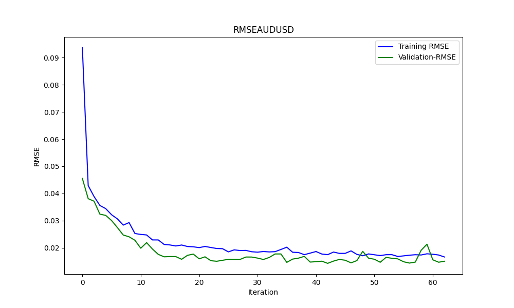
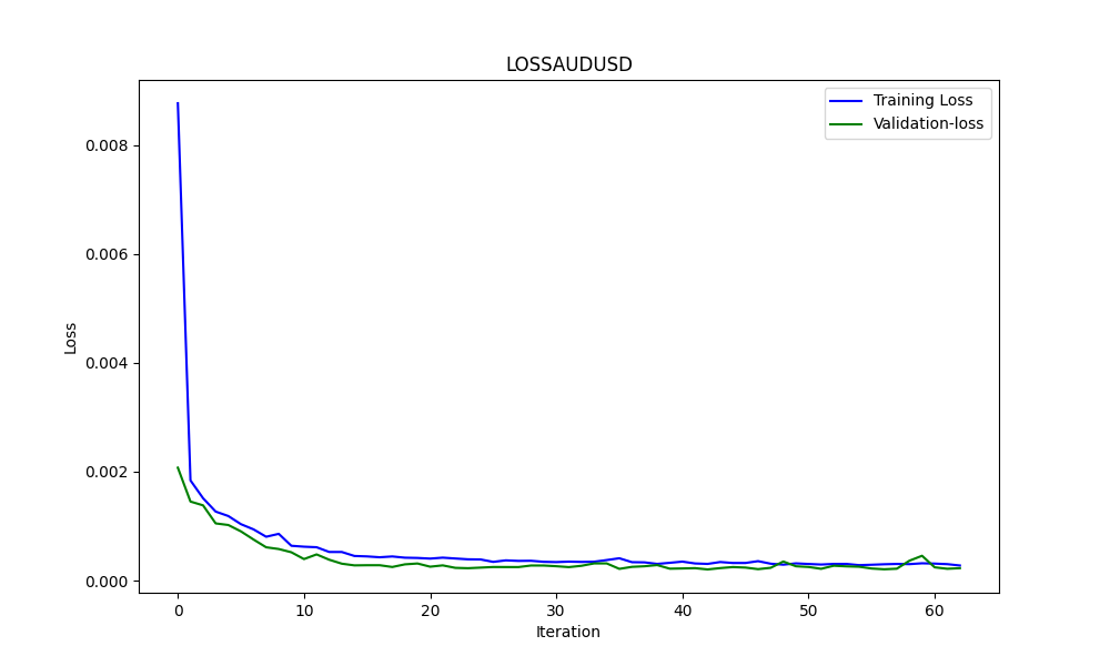
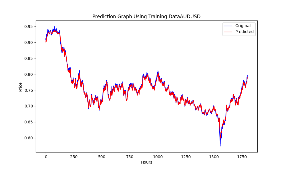
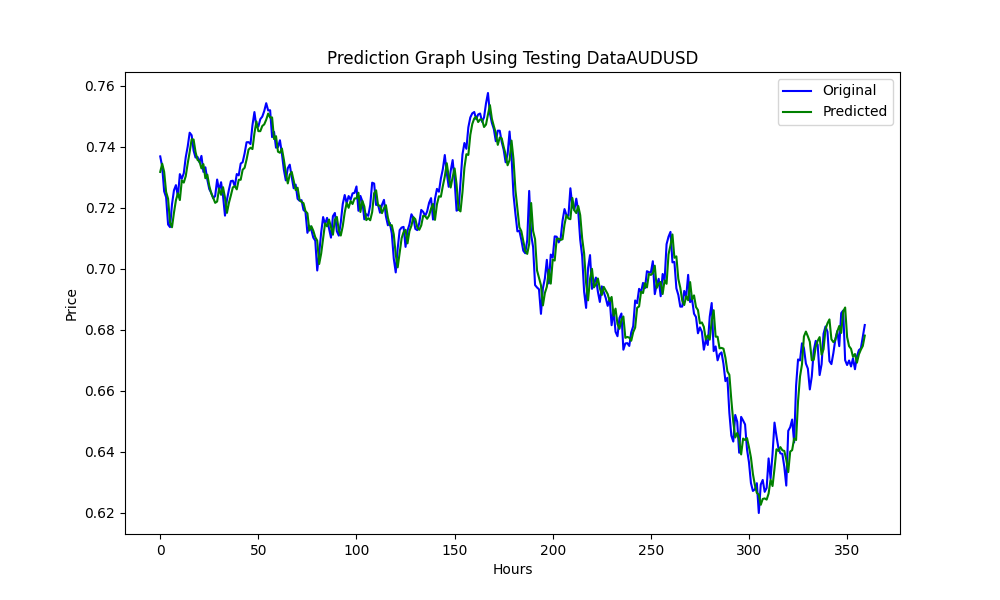
結果は

0.005679790676089899
3.226002212419775e-05
0.9670613229880559

です。それぞれRMSE、MSE、R2です。

Pythonによるバックテスト

以下の.pyを使い、戦略を変更し、バックテストの結果を確認することができます：

import MetaTrader5 as mt5
import pandas as pd
from scipy.stats import pearsonr
from statsmodels.tsa.stattools import coint
import numpy as np


# Función para la estrategia de Pairs Trading
def pairs_trading_strategy(data0, data1):
    spread = data0 - data1
    short_entry = np.mean(spread) - 2 * np.std(spread)
    short_exit = np.mean(spread)
    long_entry = np.mean(spread) + 2 * np.std(spread)
    long_exit = np.mean(spread)

    positions = []
    for i in range(len(spread)):
        if spread[i] > long_entry and (not positions or positions[-1][1] != 1):
            positions.append((spread[i], 1))
        elif spread[i] < short_entry and (not positions or positions[-1][1] != -1):
            positions.append((spread[i], -1))
        elif spread[i] < long_exit and positions and positions[-1][1] == 1:
            positions.append((spread[i], 0))
        elif spread[i] > short_exit and positions and positions[-1][1] == -1:
            positions.append((spread[i], 0))

    return positions


# Conectar con MetaTrader 5
if not mt5.initialize():
    print("No se pudo inicializar MT5")
    mt5.shutdown()

# Obtener la lista de símbolos
symbols = mt5.symbols_get()
symbols = [s.name for s in symbols if 'EUR' in s.name or 'USD' in s.name]  # Filtrar símbolos

data = {}
for symbol in symbols:
    rates = mt5.copy_rates_from_pos(symbol, mt5.TIMEFRAME_D1, 0, 365)
    if rates is not None:
        df = pd.DataFrame(rates)
        df['time'] = pd.to_datetime(df['time'], unit='s')  # Convertir a datetime
        df.set_index('time', inplace=True)
        data[symbol] = df['close']

mt5.shutdown()

# Identificar pares cointegrados
cointegrated_pairs = []
for i in range(len(symbols)):
    for j in range(i + 1, len(symbols)):
        if symbols[i] in data and symbols[j] in data:
            common_index = data[symbols[i]].index.intersection(data[symbols[j]].index)
            if len(common_index) > 30:
                corr, _ = pearsonr(data[symbols[i]][common_index], data[symbols[j]][common_index])
                if abs(corr) > 0.8:
                    score, p_value, _ = coint(data[symbols[i]][common_index], data[symbols[j]][common_index])
                    if p_value < 0.05:
                        cointegrated_pairs.append((symbols[i], symbols[j], corr, p_value))

print(cointegrated_pairs)

# Ejecutar estrategia de Pairs Trading para pares cointegrados
for sym1, sym2, _, _ in cointegrated_pairs:
    positions = []
    df0 = data[sym1]
    df1 = data[sym2]

    positions = pairs_trading_strategy(df0.values, df1.values)

    print(f'Backtesting completed for pair: {sym1} - {sym2}')
    print('Positions:', positions)

MT5ストラテジーテスターによるバックテスト

ONNXのモデルができたら、EAを動かすことができます。私はシンプルなストラテジーを使用することにしましたが、ご自分に必要な戦略をご自由にご選択ください。結果と戦略を示すことができれば幸いです。

最初にこれをおこなったとき、NZDUSDとAUDUSDは共和分で相関していましたが、現時点ではフィルターを通過しません (共和分は0.05未満)。教育目的で、また、ONNXモデルを再び作る必要がないように、この2つの銘柄で続けることにします。

//+------------------------------------------------------------------+
//|                               Hybrid Arbitrage_Statistic ONNX.mq5|
//|           Copyright 2024, Javier S. Gastón de Iriarte Cabrera. |
//|                      https://www.mql5.com/ja/users/jsgaston/news |
//+------------------------------------------------------------------+
#property copyright   "Copyright 2024, Javier S. Gastón de Iriarte Cabrera."
#property link        "https://www.mql5.com/ja/users/jsgaston/news"
#property version     "1.00"

#property strict
#include <Trade\Trade.mqh>
input double lotSize = 0.1;
//input double slippage = 3;
input double stopLoss = 1500;
input double takeProfit = 1500;
//input double maxSpreadPoints = 10.0;

#resource "/Files/art/hybrid/NZDUSD_D1.onnx" as uchar ExtModel[]
#resource "/Files/art/hybrid/AUDUSD_D1.onnx" as uchar ExtModel2[]

#define SAMPLE_SIZE 120

string symbol1 = _Symbol;
input string symbol2 = "AUDUSD";
ulong ticket1 = 0;
ulong ticket2 = 0;
input bool isArbitrageActive = true;
CTrade ExtTrade;
double spreads[1000]; // Array para almacenar hasta 1000 spreads
int spreadIndex = 0; // Índice para el próximo spread a almacenar

long     ExtHandle=INVALID_HANDLE;
//int      ExtPredictedClass=-1;
datetime ExtNextBar=0;
datetime ExtNextDay=0;
float    ExtMin=0.0;
float    ExtMax=0.0;


long     ExtHandle2=INVALID_HANDLE;
//int      ExtPredictedClass=-1;
datetime ExtNextBar2=0;
datetime ExtNextDay2=0;
float    ExtMin2=0.0;
float    ExtMax2=0.0;

float predicted=0.0;
float predicted2=0.0;

float   lastPredicted1=0.0;
float   lastPredicted2=0.0;

int Order=0;
//+------------------------------------------------------------------+
//| Expert initialization function                                   |
//+------------------------------------------------------------------+
int OnInit()
  {
   Print("EA de arbitraje ONNX iniciado");

//--- create a model from static buffer
   ExtHandle=OnnxCreateFromBuffer(ExtModel,ONNX_DEFAULT);
   if(ExtHandle==INVALID_HANDLE)
     {
      Print("OnnxCreateFromBuffer error ",GetLastError());
      return(INIT_FAILED);
     }

//--- since not all sizes defined in the input tensor we must set them explicitly
//--- first index - batch size, second index - series size, third index - number of series (only Close)
   const long input_shape[] = {1,SAMPLE_SIZE,1};
   if(!OnnxSetInputShape(ExtHandle,ONNX_DEFAULT,input_shape))
     {
      Print("OnnxSetInputShape error ",GetLastError());
      return(INIT_FAILED);
     }

//--- since not all sizes defined in the output tensor we must set them explicitly
//--- first index - batch size, must match the batch size of the input tensor
//--- second index - number of predicted prices (we only predict Close)
   const long output_shape[] = {1,1};
   if(!OnnxSetOutputShape(ExtHandle,0,output_shape))
     {
      Print("OnnxSetOutputShape error ",GetLastError());
      return(INIT_FAILED);
     }


//--- create a model from static buffer
   ExtHandle2=OnnxCreateFromBuffer(ExtModel2,ONNX_DEFAULT);
   if(ExtHandle2==INVALID_HANDLE)
     {
      Print("OnnxCreateFromBuffer error ",GetLastError());
      return(INIT_FAILED);
     }

//--- since not all sizes defined in the input tensor we must set them explicitly
//--- first index - batch size, second index - series size, third index - number of series (only Close)
   const long input_shape2[] = {1,SAMPLE_SIZE,1};
   if(!OnnxSetInputShape(ExtHandle2,ONNX_DEFAULT,input_shape2))
     {
      Print("OnnxSetInputShape error ",GetLastError());
      return(INIT_FAILED);
     }

//--- since not all sizes defined in the output tensor we must set them explicitly
//--- first index - batch size, must match the batch size of the input tensor
//--- second index - number of predicted prices (we only predict Close)
   const long output_shape2[] = {1,1};
   if(!OnnxSetOutputShape(ExtHandle2,0,output_shape2))
     {
      Print("OnnxSetOutputShape error ",GetLastError());
      return(INIT_FAILED);
     }



   return(INIT_SUCCEEDED);
  }

//+------------------------------------------------------------------+
//| Expert deinitialization function                                 |
//+------------------------------------------------------------------+
void OnDeinit(const int reason)
  {
   if(ExtHandle!=INVALID_HANDLE)
     {
      OnnxRelease(ExtHandle);
      ExtHandle=INVALID_HANDLE;
     }

   if(ExtHandle2!=INVALID_HANDLE)
     {
      OnnxRelease(ExtHandle2);
      ExtHandle2=INVALID_HANDLE;
     }
  }

//+------------------------------------------------------------------+
//| Expert tick function                                             |
//+------------------------------------------------------------------+
void OnTick()
  {
//--- check new day
   if(TimeCurrent()>=ExtNextDay)
     {
      GetMinMax();
      GetMinMax2();
      //--- set next day time
      ExtNextDay=TimeCurrent();
      ExtNextDay-=ExtNextDay%PeriodSeconds(PERIOD_D1);
      ExtNextDay+=PeriodSeconds(PERIOD_D1);
      /*ExtTrade.PositionClose(symbol1);
      ExtTrade.PositionClose(symbol2);
      ticket1 = 0;
      ticket2 = 0;*/
     }

//--- check new bar
   if(TimeCurrent()<ExtNextBar)
     {

      return;
     }
//--- set next bar time
   ExtNextBar=TimeCurrent();
   ExtNextBar-=ExtNextBar%PeriodSeconds();
   ExtNextBar+=PeriodSeconds();
//--- check min and max
   float close=(float)iClose(symbol1,PERIOD_D1,0);
   if(ExtMin>close)
      ExtMin=close;
   if(ExtMax<close)
      ExtMax=close;
   float close2=(float)iClose(symbol2,PERIOD_D1,0);
   if(ExtMin2>close2)
      ExtMin2=close2;
   if(ExtMax2<close2)
      ExtMax2=close2;

   lastPredicted1=predicted;
   lastPredicted2=predicted2;

//--- predict next price
   PredictPrice();
   PredictPrice2();



   if(!isArbitrageActive || ArePositionsOpen())
     {
      Print("Arbitraje inactivo o ya hay posiciones abiertas.");
      return;
     }
   double price1 = SymbolInfoDouble(symbol1, SYMBOL_BID);
   double price2 = SymbolInfoDouble(symbol2, SYMBOL_ASK);
   double currentSpread = MathAbs(price1 - price2);
   Print("current spread ", currentSpread);
   Print("Price1 ",price1);
   Print("Price2 ",price2);
   Print("PricePredicted1 ",predicted);
   Print("PricePredicted2 ",predicted2);
   Print("Last PricePredicted1 ",lastPredicted1);
   Print("Last PricePredicted2 ",lastPredicted2);

   double predictedSpread = MathAbs(predicted - predicted2);
   Print("Predicted spread ", predictedSpread);

   double LastpredictedSpread = MathAbs(lastPredicted1 - lastPredicted2);
   Print("Last Predicted spread ", LastpredictedSpread);

// Almacenar el spread actual en el array y actualizar el índice
   spreads[spreadIndex % 1000] = currentSpread;
   spreadIndex++;

// Verifica si hay suficientes datos para calcular la desviación estándar
   int count = MathMin(spreadIndex, 1000); // Utiliza todos los datos disponibles hasta 1000
   double stdDevSpread = CalculateStdDev(spreads, 0, count);
//Print("StdDevSpread ", stdDevSpread);

// Verifica si el spread es lo suficientemente bajo para el arbitraje
   if(LastpredictedSpread< currentSpread)
     {
      // Inicia el arbitraje si aún no está activo
      if(isArbitrageActive)
        {
         //Print("max spread : ",maxSpreadPoints * _Point);
         double meanSpread = (lastPredicted1 + lastPredicted2) / 2.0;
         Print("mean spread: ",meanSpread);
         double stdDevSpread = CalculateStdDev(spreads, 0, ArraySize(spreads));
         Print("StdDevSpread ", stdDevSpread);
         double shortEntry = meanSpread - 2 * stdDevSpread ;

         double shortExit = meanSpread;
         double longEntry = meanSpread + 2 * stdDevSpread ;

         double longExit = meanSpread;

         Print("Long Entry: ", longEntry, " Short Entry: ", shortEntry);

         // Comprueba si la condición de entrada corta se cumple para el arbitraje
         if(price1 < shortEntry && (ticket1 == 0 || ticket2 == 0))
           {
            Print("Preparando para abrir órdenes");
            Order = 1;


            Print("Error al abrir posiciones de arbitraje: ", GetLastError());
            ticket1 = ExtTrade.PositionOpen(symbol1, ORDER_TYPE_BUY, lotSize, price1, price1 - stopLoss * _Point, price1 + takeProfit * _Point, "Arbitraje");
            ticket2 = ExtTrade.PositionOpen(symbol2, ORDER_TYPE_SELL, lotSize, price2, price2 + stopLoss * _Point, price2 - takeProfit * _Point, "Arbitraje");
            ticket1=0;
            ticket2=0;
           }
         else
            if(price2 < shortEntry && (ticket1 == 0 || ticket2 == 0))
              {
               Print("Preparando para abrir órdenes");
               Order = 2;


               Print("Error al abrir posiciones de arbitraje: ", GetLastError());
               ticket1 = ExtTrade.PositionOpen(symbol1, ORDER_TYPE_SELL, lotSize, price1, price1 + stopLoss * _Point, price1 - takeProfit * _Point, "Arbitraje");
               ticket2 = ExtTrade.PositionOpen(symbol2, ORDER_TYPE_BUY, lotSize, price2, price2 - stopLoss * _Point, price2 + takeProfit * _Point, "Arbitraje");
               ticket1=0;
               ticket2=0;
              }

            else
               if(price1 > longEntry && (ticket1 == 0 || ticket2 == 0))
                 {
                  Print("Preparando para abrir órdenes");
                  Order = 3;


                  Print("Error al abrir posiciones de arbitraje: ", GetLastError());
                  ticket1 = ExtTrade.PositionOpen(symbol1, ORDER_TYPE_SELL, lotSize, price1, price1 + stopLoss * _Point, price1 - takeProfit * _Point, "Arbitraje");
                  ticket2 = ExtTrade.PositionOpen(symbol2, ORDER_TYPE_BUY, lotSize, price2, price2 - stopLoss * _Point, price2 + takeProfit * _Point, "Arbitraje");
                  ticket1=0;
                  ticket2=0;
                 }
               else
                  if(price2 > longEntry && (ticket1 == 0 || ticket2 == 0))
                    {
                     Print("Preparando para abrir órdenes");
                     Order = 4;


                     Print("Error al abrir posiciones de arbitraje: ", GetLastError());

                     ticket1 = ExtTrade.PositionOpen(symbol1, ORDER_TYPE_BUY, lotSize, price1, price1 - stopLoss * _Point, price1 + takeProfit * _Point, "Arbitraje");
                     ticket2 = ExtTrade.PositionOpen(symbol2, ORDER_TYPE_SELL, lotSize, price2, price2 + stopLoss * _Point, price2 - takeProfit * _Point, "Arbitraje");
                     ticket1=0;
                     ticket2=0;
                    }

        }
     }
//+------------------------------------------------------------------+
//|                                                                  |
//+------------------------------------------------------------------+
   double meanSpread = (lastPredicted1 + lastPredicted2) / 2.0;
//Print("mean spread: ",meanSpread);
   double stdDevSpread2 = CalculateStdDev(spreads, 0, ArraySize(spreads));
//Print("StdDevSpread ", stdDevSpread);
   double shortEntry = meanSpread - 2 * stdDevSpread2 ;

   double shortExit = meanSpread;
   double longEntry = meanSpread + 2 * stdDevSpread2 ;

   double longExit = meanSpread;
   if((price2 < longExit && ticket2 != 0 && Order==4) || (price1 > shortExit && ticket1 != 0 && Order==1) || (price2 > shortExit && ticket1 != 0 && Order==2) || (price1 < longExit && ticket2 != 0 && Order==3))
     {
      ExtTrade.PositionClose(ticket1);
      ExtTrade.PositionClose(ticket2);
      ticket1 = 0;
      ticket2 = 0;
      Print("Arbitraje detenido - Cerrando órdenes");
     }

  }

//+------------------------------------------------------------------+
//|                                                                  |
//+------------------------------------------------------------------+
double CalculateStdDev(double &data[], int start, int count)
  {
   double sum = 0;
   double sumSq = 0;
   for(int i = start; i < start + count; i++)
     {
      sum += data[i];
      sumSq += data[i] * data[i];
     }
   double mean = sum / count;
   double variance = (sumSq / count) - (mean * mean);
   return MathSqrt(variance);
  }
//+------------------------------------------------------------------+
//|                                                                  |
//+------------------------------------------------------------------+
bool ArePositionsOpen()
  {
// Check for positions on symbol1
   if(PositionSelect(symbol1) && PositionGetDouble(POSITION_VOLUME) > 0)
      return true;
// Check for positions on symbol2
   if(PositionSelect(symbol2) && PositionGetDouble(POSITION_VOLUME) > 0)
      return true;

   return false;
  }
//+------------------------------------------------------------------+
void PredictPrice(void)
  {
   static vectorf output_data(1);            // vector to get result
   static vectorf x_norm(SAMPLE_SIZE);       // vector for prices normalize

//--- check for normalization possibility
   if(ExtMin>=ExtMax)
     {
      Print("ExtMin>=ExtMax");
      //ExtPredictedClass=-1;
      return;
     }
//--- request last bars
   if(!x_norm.CopyRates(_Symbol,PERIOD_D1,COPY_RATES_CLOSE,1,SAMPLE_SIZE))
     {
      Print("CopyRates ",x_norm.Size());
      //ExtPredictedClass=-1;
      return;
     }
   float last_close=x_norm[SAMPLE_SIZE-1];
//--- normalize prices
   x_norm-=ExtMin;
   x_norm/=(ExtMax-ExtMin);
//--- run the inference
   if(!OnnxRun(ExtHandle,ONNX_NO_CONVERSION,x_norm,output_data))
     {
      Print("OnnxRun");
      //ExtPredictedClass=-1;
      return;
     }
//--- denormalize the price from the output value
   predicted=output_data[0]*(ExtMax-ExtMin)+ExtMin;
//return predicted;
  }
//+------------------------------------------------------------------+
//|                                                                  |
//+------------------------------------------------------------------+
void PredictPrice2(void)
  {
   static vectorf output_data2(1);            // vector to get result
   static vectorf x_norm2(SAMPLE_SIZE);       // vector for prices normalize

//--- check for normalization possibility
   if(ExtMin2>=ExtMax2)
     {
      Print("ExtMin2>=ExtMax2");
      //ExtPredictedClass=-1;
      return;
     }
//--- request last bars
   if(!x_norm2.CopyRates(symbol2,PERIOD_D1,COPY_RATES_CLOSE,1,SAMPLE_SIZE))
     {
      Print("CopyRates ",x_norm2.Size());
      //ExtPredictedClass=-1;
      return;
     }
   float last_close2=x_norm2[SAMPLE_SIZE-1];
//--- normalize prices
   x_norm2-=ExtMin2;
   x_norm2/=(ExtMax2-ExtMin2);
//--- run the inference
   if(!OnnxRun(ExtHandle2,ONNX_NO_CONVERSION,x_norm2,output_data2))
     {
      Print("OnnxRun");
      //ExtPredictedClass=-1;
      return;
     }
//--- denormalize the price from the output value
   predicted2=output_data2[0]*(ExtMax2-ExtMin2)+ExtMin2;
//--- classify predicted price movement
//return predicted2;
  }

//+------------------------------------------------------------------+
//| Get minimal and maximal Close for last 120 days                  |
//+------------------------------------------------------------------+
void GetMinMax(void)
  {
   vectorf close;
   close.CopyRates(_Symbol,PERIOD_D1,COPY_RATES_CLOSE,0,SAMPLE_SIZE);
   ExtMin=close.Min();
   ExtMax=close.Max();
  }

//+------------------------------------------------------------------+
//| Get minimal and maximal Close for last 120 days                  |
//+------------------------------------------------------------------+
void GetMinMax2(void)
  {
   vectorf close2;
   close2.CopyRates(symbol2,PERIOD_D1,COPY_RATES_CLOSE,0,SAMPLE_SIZE);
   ExtMin2=close2.Min();
   ExtMax2=close2.Max();
  }

以下は、1分足のNZDUSDとAUDUSDの結果です。ONNXモデルは1日足で、SLは1500ポイント、TPは1500ポイントで、2023年1月1日から2024年1月1日までを予測するモデルを使用しています。

フィルターする他のペアを選択するには、この行を変更します。

symbols = [s.name for s in symbols if s.name.startswith('EUR') or s.name.startswith('USD') or s.name.endswith('USD')]

ケーススタディ2

裁定取引は株式取引で非常によく使用されます。だからこそ、ナスダックのペアを使用した別の例は興味深いです。

私の場合、次の行

symbols = [s.name for s in symbols if s.name.startswith('EUR') or s.name.startswith('USD') or s.name.endswith('USD')]

を次のように変更しました。

# Crea un DataFrame con la información completa de los símbolos
symbols_df = pd.DataFrame([{'Symbol': symbol.name, 'Path': symbol.path} for symbol in all_symbols])

# Filtra adicionalmente para obtener solo los CFDs de NASDAQ
# Asumiendo que los CFDs tienen un identificador único en el 'Path'
nasdaq_group4_df = symbols_df[symbols_df['Path'].str.contains('NASDAQ')]

# Filtra aún más para obtener solo los símbolos que NO contienen '.'
nasdaq_group4_df3 = nasdaq_group4_df[nasdaq_group4_df['Symbol'].str.contains('#')]

nasdaq_group4_df2 = nasdaq_group4_df3[~nasdaq_group4_df3['Symbol'].str.contains('\.')]

# Ahora, obtenemos la lista de símbolos filtrados
filtered_symbols = nasdaq_group4_df2['Symbol'].tolist()
# Descargar datos históricos y almacenar en un diccionario
symbols = filtered_symbols

ここでペアのフィルターがかかります。

非常に多くのペアが共和分で相関したので、スクリプトを変更しなければなりませんでした（.pyを修正してこれをcsvで出力する）。

変更

# Filtrar y guardar solo los pares cointegrados con p-valor menor de 0.05 en un archivo CSV
result_df = pd.DataFrame(cointegrated_pairs, columns=['Symbol1', 'Symbol2', 'Correlation', 'Cointegration P-value'])
result_df.to_csv('cointegrated_pairs.csv', index=False)

# Imprimir el total de pares cointegrados
print(f'Total de pares con fuerte correlación y cointegrados: {len(cointegrated_pairs)}')

これは、NASDAQからフィルタリングされたペアです。

当面は、アマゾンとネットフリックスについて、2023年1月1日から2024年1月1日までの予測モデルで説明します。

#AMZN   #NFLX   0.966605859     0.021683012

より良い結果を得るために、サンプル数を3倍にしました。

sample_size = 120*25*3

結果はこうです。

6.856399020501732
47.010207528337105
0.9395402850007741 

25.975755379462548
674.7398675336775
0.9735838717570285 

SLは400、TPは800

そしてSLとTPを微調整し、素早く最適化した結果がこれです。

すべてのスクリプトとONNXをダウンロードするEAとして残しました。これを体系的かつ科学的に使用することで、同じ結果を得ることができます。必要な日付に新しいONNXを作成し（.py の訓練の日付を変更することを忘れないでください）、ストラテジーテスターの日付も変更します。例：D1期間のONNXモデルと120*3*25のデータは、最大で1年間使用することができます（ただし、私だったら、週または月ごとに作成します）。

覚えておいていただきたいのは、これはあくまで例を挙げた戦略であって、取引に使用するためのボットをすぐに構築できるものではないし、インターネット上で無料で見つかることもおそらくないだろう、ということです。

結論

相関と共和分の使い方を見てきましたが、最終的にはピアソン係数の指標と予測を使用した裁定取引のEAを手に入れることになりました。.pyフィルターから正しいペアを使用すると、より良い結果が得られます。より良い結果を得るためにSLとTPを微調整し、戦略をより複雑にすることができます。 

ONNXモデルはMQL5/Filesフォルダ、mq5指標はIndicatorフォルダ、EAはEAのフォルダ(Experts)に保存することをお忘れなく。