Error gradient backpropagation method

Once we have defined the loss function, we can move on to training the neural network. The actual learning process involves iteratively adjusting the neural network parameters (synaptic weights) at which the value of the neural network loss function will be minimized.

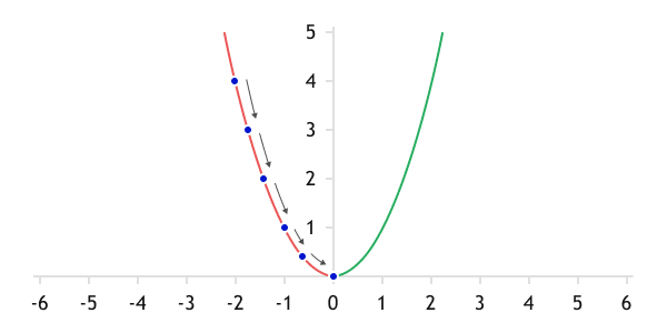
From the previous section, we learned that the loss function is concave downward. Therefore, when starting the training from any point on the loss function graph, we should move in the direction of minimizing the error. For complex functions like a neural network, the most convenient method is the gradient descent algorithm.

The gradient of a multi-variable function (which a neural network is) is defined as a vector composed of the partial derivatives of the function with respect to its arguments. From our mathematics course, we know that the derivative of a function characterizes the rate of change of the function at a given point.

Hence, the gradient indicates the direction of the fastest growth of the function. Moving in the direction of the negative gradient (opposite to the gradient), we will descend at the maximum speed towards the minimum of the function.

The algorithm of action will be as follows:

1. Initialize the weights of the neural network using one of the ways described earlier.
2. Compute the predicted data on the training sample.
3. Using the loss function, calculate the computational error of the neural network.
4. Determine the gradient of the loss function at the obtained point.
5. Adjust the synaptic coefficients of the neural network towards the negative gradient.

Since a nonlinear loss function is used often, the direction of the anti-gradient vector will change at each point on the loss function graph. Therefore, we will reduce the loss function gradually, getting closer and closer to the minimum with each iteration.

At first glance, the algorithm is quite simple and logical. But how do we technically implement point 5 of our algorithm in the case of a multilayer neural network?

This issue is addressed using the backpropagation algorithm, which consists of two main components:

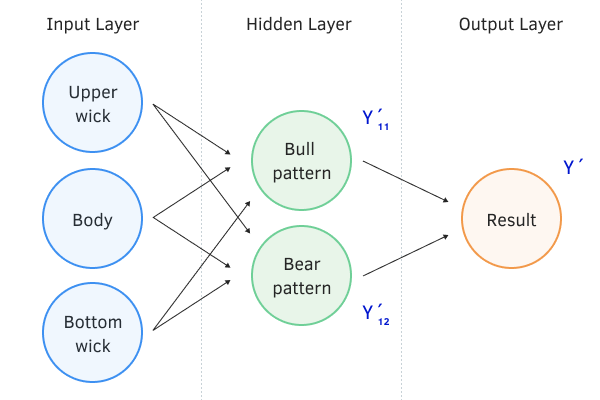
1. Forward pass. Point 2 from our algorithm above. During the forward pass, a set of data from the training sample is fed to the input of the neural network and processed in the neural network sequentially from the input layer to the output layer. The intermediate values on each neuron are preserved.

2. The backward pass includes steps 3-5 of our algorithm.

At this point, it's worth recalling some mathematics. We talk about partial derivatives of a function, but we also want to train a neural network that consists of a large number of neurons. At the same time, each neuron represents a complex function, and to update the weights of the neural network, we need to calculate the partial derivatives of the composite function of our neural network with respect to each weight.

According to the rules of mathematics, the derivative of a composite function is equal to the product of the derivative of the outer function and the derivative of the inner function.

Let us use this rule and find the partial derivatives of the loss function L by the weight of the output neuron wi and by the ith input value xi.

Where:

• L = loss function
• A = activation function of the neuron
• S = weighted sum of the raw data
• X = vector of initial data
• W = vector of weights
• wi = ith weighting factor for which the derivative is calculated
• xi = ith element of the initial data vector

The first thing to notice in the formulas presented above is the complete coincidence of the first two multipliers. I.e., when calculating partial derivatives on weights and initial data, we only need to calculate the error gradient in front of the activation function once, and using this value, calculate partial derivatives for all elements of the vectors of weights and initial data.

Using a similar method, we can determine the partial derivative with respect to the weight of one of the neurons in the hidden layer that precedes the output neuron layer. For this purpose, in the previous formula we replace the vector of initial data with the function of the hidden layer neuron. The vector of weights will be transformed into a scalar value of the corresponding weight.

Where:

• Ah = activation function of the hidden layer neuron
• Sh = weighted sum of the original data of the hidden layer neuron
• Xh = vector of initial data for the hidden layer neuron
• Wh = vector of weights of the hidden layer neuron
• wh = weight of the hidden layer for which the derivative is calculated

Note that if in the last formula, we return X instead of the function of the hidden layer neuron, we see in the first function multipliers the function of the private derivative of the ith input value presented above.

Hence,

Similar formulas can be provided for each neuron in our network. Thus, we can calculate the derivative and error gradient of the neuron output once, and then propagate the error gradient to all the connected neurons in the previous layer.

Following this logic, we first determine the deviations from the reference value using the loss function. The loss function can be anything that satisfies the requirements described in the previous section.

,

Where:

• Y = vector of reference values
• Y' = vector of values at the output of the neural network

Next, we determine how the states of the neurons in the output layer should change in order for our loss function to reach its minimum value. From a mathematical perspective, we determine the error gradient on each neuron in the output layer by calculating the partial derivative of the loss function with respect to each parameter.

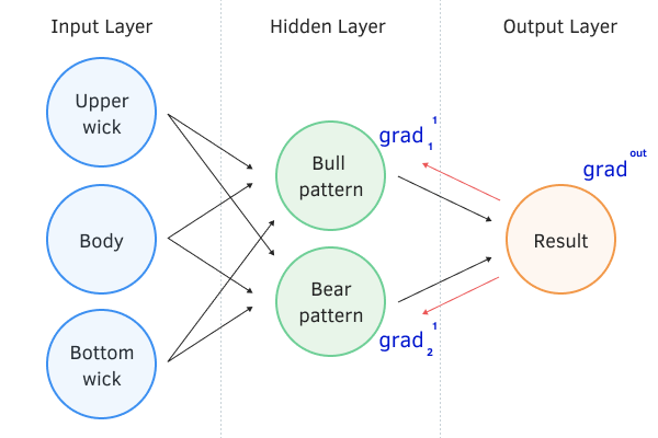
We then "descend" the error gradient from the output neural layer to the input layer by running it sequentially through all the hidden neural layers of our network. In this way, we are effectively bringing the reference value to each neuron at this stage of training.

Where:

• gradij–1 = gradient at the output of the ith neuron of the j–1 layer
• Akj = the activation function of the kth neuron on the jth layer
• Skj = weighted sum of incoming data of the kth neuron on the jth layer
• Wkj = vector of synaptic coefficients of the kth neuron on the jth layer

After obtaining the error gradients at the output of each neuron, we can proceed to adjust the synaptic coefficients of the neurons. For this purpose, we will go through all layers of the neural network one more time. At each layer, we will search all neurons and for each neuron, we will update all synaptic connections.

We will talk about ways to update the weights in the next chapter.

After updating the weights, we return to step 2 of our algorithm. The cycle is repeated until the minimum of the function is found. Determining the achievement of the minimum can be done by observing zero partial derivatives. In general, it will be noticeable by the absence of change of the error at the output of the neural network after the next cycle of updating the weights, because at zero derivatives the process of training of the neural network stops.