Category Theory in MQL5 (Part 21): Natural Transformations with LDA

Introduction

So far, we have covered quite a number of topics in category theory that easily lean towards applicability outside of their academic setting. If I may list a few of these, they’ve included: sets & morphisms, commutation, ontology logs, products, coproducts, limits, colimits, monoids, groups, graphs, orders, functors, and now natural transformations. Category theory is much wider than what we have considered here and these topics are selected for their easy applicability and use in other disciplines related to Mathematics. If you’re interested in a more thorough review of the subject, this book, which some regard as the Bible in these matters should be interesting.

As we continue our look at natural transformations we will for this article look at more applications in time series forecasting. Natural transformations can often be inferred in data sets that are related and this is something we want to start looking at with this article.

So, here is the problem. A startup company creates a database for its customers to keep track of their purchases over time and initially it has let’s say, 3 columns. A primary key, a product name column, and an amount paid column. Over time the company notices a lot of repetition in the product column, meaning a particular product is getting bought a lot. So, in response to this a decision is made to start logging more information related to products so as to better distinguish the preferences of the customer and possibly explore developing new products that may be missing from their portfolio. To this end the product column gets split into 3 columns namely: version, subscription mode, build name. Or the company may need more color on the payment information and decide to partition the payment column into 3 with say a column for payment mode, currency (or locale), and the payment amount. Again, such splits would not be exhaustive as at a future stage more may be required depending on the customer purchases and their preferences.

Each of these new created columns would map to the old product column. And if we had, for example, established some key correlations between the old single product column and say the amount paid column, or any other column in a table within the database, then it would be a cumbersome process in re-establishing these correlations in the new table structure. The startup company would certainly have many means of addressing this but natural transformations do offer a seamless alternative.

To wrap our heads around this let’s try to look at this firstly as two categories. In the domain category we would have the startup company’s list of tables in its database, and in the codomain category we would have the two versions of the customer information tables. For simplicity if we take the list as a single object in the domain and each of our tables as separate objects in the codomain then two functors from the list one to each table, do imply a natural transformation between the two tables. So, one functor would map to old tables which in our case is the simple 3 column table, while the second functor would map to a revision in the table structure. If this is revision 1 then the second functor maps to the 5-column table.

The implication of a natural transformation not only means we can quantify the differences between these two tables via an algorithmic mapping function such as: linear equation, quadratic equation, multi-layer perceptron, random distribution forest, or linear discriminant analysis; it means we can use these weights to re-establish prior correlations with the old table and develop new ones for the created columns.

Background

So just to briefly recap natural transformations are the difference between the target objects of two functors. The use of this difference has been highlighted in these series with the naturality square, a commutative composition of objects in the codomain category of these functors. We introduced this in article 18 and also looked at further examples of this with naturality square induction in article 19.

The concept of time-series data is not alien to most traders as many of us are not just familiar with price charts, and in-built indicators of MetaTrader terminal, but many traders do code their own custom indicators and also develop their expert advisors. So some groundwork on subjects like these and these has been covered by most people. Nonetheless the price of say a forex pair as viewed on a chart is a discrete-time series given that we have a definite price at each interval, this is despite the fact, when the markets are open which is most of the week, this price will always be changing meaning it really is a continuous-time series. So, the discrete-time series view is used to help with analysis.

The ability to perform analysis therefore is rooted in having ‘consensus’ prices for a given security at a particular time. And when trying to make forecasts which tends to be the objective of most forecasts, the study of different series at different time epochs becomes important. That is why looking at and comparing data with a time lag can be seen as more constructive in getting accurate results.

Thus, for this article we will look at two datasets, as hinted at in the intro they will be similar with one simply more elaborate than the other. With these two sets we will have them in a lagged natural transformation so as to aid with making projections. Our two datasets, which can be represented as tables, will be very simple. The first will feature moving average values while the second will have the constituent prices of this average.

Data Sets Description

So, the simple table will have just two columns. A timestamp column and a moving average column. The number of rows in this and the compound table will be set by the user with input parameter ‘m_data’. This simple table will be staggered ahead in time to the compound table by the size of the moving average period used. So, if our moving average period is 5 then the values in this table will be 5-time bars of the compound table.

The compound table that is the laggard will also have a time stamp column and more columns each with a price at a different point in time. The number of these extra columns beyond the time stamp will be set by the moving average period so once again if our moving average is over 5 price bars then this table will have one-time stamp column and 5 price columns.

These two datasets that have a natural transformation mapping can have this defined in a number of ways as listed already in the introduction. For this article we will use a method we are yet to consider in these series and that is the linear discriminant analysis (LDA). I had shown how this could be used with the MQL5 wizard and the Alglib library in this article nonetheless it may be helpful to do a recap here.

A more concrete definition of this can be found here but broadly LDA is a classifier. If we look at any typical training dataset, it always has independent variables (values that are hypothesized to influence the end result) and classifier variable(s) which serve as the ‘end result’. With LDA we have ability to pigeonhole this end result in up to n classes where n in a natural number. This algorithm that was developed by Sir Ronald Fisher outputs a vector of weights that help define the main centroid of each classifier and can also estimate the position of an unknown centroid (new or unknown data point). With this information one can simply compare the position of the unknown centroid to that of the known to know which it is closer to and therefore what its classification is. To illustrate this a ‘vector of weights’ could be thought of as an equation to a line that separates points that have only 2 classifiers. If the classifiers are three then it is the equation of a plane. If one then it is the coordinates on a number line. In either scenario you are able to draw distinction among a training data set by giving each data point a set of coordinates.

Natural Transformation for Time-Series Forecasting

So, as we mentioned in previous articles 18, and 19 when looking at naturality squares usually the codomain objects are all that matter and that’s why in showing how two different datasets of price points and moving averages can share a natural transformation for this article, we have not said anything about the functor source category or object(s). They are not critical. If we however have multiple objects in the source category then you would expect multiple pro-rata instances of both the simple data set and the compound data set. This was highlighted when we saw naturality square induction in article 19.

So, from a diagram mapping perspective our natural transformation should not be overly complicated. The time stamp columns of the datasets would be linked and all the price columns in the compound dataset would map to the moving average column in the simple dataset. This is usually represented in MQL5 code for illustration and logic reasons and to that end we have instances of the simple dataset and compound datasets declared as ‘m_o_s’ and ‘m_o_c’ respectively. These class instances are now named ‘objects’ and not ‘domains’ in recognition of the term ‘domain’ being a property to one of morphism linked objects and not necessarily a noun in itself. (if that makes sense). What I referred to as a domain in most of our earlier articles is more commonly called an object. I had refrained from using ‘object’ to avoid confusion with the inbuilt classes of MQL5. This approach is less error prone to mistakes in logic that could easily be made if we were more direct and copied price data directly to our mapping function. These are the sort of bugs that do not show up even when testing the expert because it compiles normally thus we are only demonstrating it here to show what is possible.

So, the natural transformation is implemented using LDA and the critical mapping will be from the lagging price points to the future moving average price value. The time stamp column will not be utilized but is mentioned for completeness so the reader can get a sense of how the data is structured. The time lag as stated above will be equivalent to the length of the moving average period. So, when training we would be using prices that are n bars back from the start index where n is the length of our moving average period. This also means when forecasting we obviously use the latest prices but our forecast would be for n bars in the future. Not the immediate moving average.

Applying the Natural Transformation for Forecasting

The code therefore for this will primarily be handled by two functions within the signal class because as stated we are not coding with the entire class structures that typically outline categories that is morphisms, or functors as we have in the past; rather we will use just the objects and elements classes to map what is in the codomain category. The end result should be identical with the approach chosen here being more efficient on computer resources and therefore easier to test in strategy tester. This though requires more care to avoid mistakes in logic of the categories and their functors as mistakes made cannot show up when you compile or run strategy tests. So, our refresh function will be as follows:

//+------------------------------------------------------------------+
//| Refresh function to update objects.                              |
//+------------------------------------------------------------------+
void CSignalCT::Refresh(int DataPoints=1)
   {
      m_time.Refresh(-1);
      m_close.Refresh(-1);
      
      for(int v=0;v<DataPoints;v++)
      {
         m_e_s.Let(); m_e_s.Cardinality(2);
         m_e_c.Let(); m_e_c.Cardinality(m_independent+1);
         
         m_e_s.Set(0,TimeToString(m_time.GetData(v)));
         m_e_c.Set(0,TimeToString(m_time.GetData(v)));
      
         double _s_unit=0.0;
         //set independent variables..
         for(int vv=0;vv<m_independent;vv++)
         {
            double _c_unit=m_close.GetData(StartIndex()+v+vv+m_independent);
            
            m_e_c.Set(vv+1,DoubleToString(_c_unit));
         }
         
         m_o_c.Set(0,m_e_c);
         
         //get dependent variable, the MA..
         for(int vv=v;vv<v+m_independent;vv++)
         {
            _s_unit+=m_close.GetData(StartIndex()+vv);
         }
         
         _s_unit/=m_independent;
         
         m_e_s.Set(1,DoubleToString(_s_unit));
         
         m_o_s.Set(0,m_e_s);
      }
   }

This refresh function will be called by the ‘get direction’ function whose listing will look as follows:

//+------------------------------------------------------------------+
//| Get Direction function from implied naturality square.           |
//+------------------------------------------------------------------+
double CSignalCT::GetDirection()
   {
      double _da=0.0;
      
      int _info=0;
      CMatrixDouble _w,_xy,_z;
      _xy.Resize(m_data,m_independent+1);
      
      double _point=0.00001;
      if(StringFind(m_symbol.Name(),"JPY")>=0){ _point=0.001; }
      
      for(int v=0;v<m_data;v++)
      {
         Refresh(v+1);
         
         ...
         
         //training classification
         _xy.Set(v,m_independent,(fabs(_ma-_lag_ma)<=m_regularizer*_point?1:(_ma-_lag_ma>0.0?2:0)));
      }
      
      m_lda.FisherLDAN(_xy,m_data,m_independent,__CLASSES,_info,_w);
      
      if(_info>0)
      {
         double _centroids[__CLASSES],_unknown_centroid=0.0; ArrayInitialize(_centroids,0.0);
         
         _z.Resize(1,m_independent+1);
         
         m_o_c.Get(0,m_e_c);
         
         for(int vv=0;vv<m_independent;vv++)
         {
            string _c="";
            m_e_c.Get(vv+1,_c);
            
            double _c_value=StringToDouble(_c);
            _z.Set(0,vv,_c_value);
         }
         
         for(int v=0;v<m_data;v++)
         {
            for(int vv=0;vv<m_independent;vv++)
            {
               _centroids[int(_xy[v][m_independent])]+= (_w[0][vv]*_xy[v][vv]);
            }
         }
         
         // best vector is the first 
         for(int vv=0;vv<m_independent;vv++){ _unknown_centroid+= (_w[0][vv]*_z[0][vv]); }
         
         
... 
      }
      else
      {
         
... 
      }
      
      return(_da);
   }

Our forecast is for a change in the future moving average price so a negative change would indicate bearishness, a positive change bullishness, and ‘no change’ would point to a flat market. On the last note to quantify ‘no change’ we have a regulizer parameter, ‘m_regulizer’, that sets the minimum forecast magnitude for it to be deemed a change for bearishness or bullishness. It is an integer that we quantify by multiplying it with the symbol’s point size.

So, this is the run-down of our code implementing the transformation. The declaration of critical variables is done as always in the class manifest. Besides the typical declarations for a signal class we add for our special class declarations for instances of a simple element, a compound element, a simple element, a compound element, an instance of our linear discriminant class.

On each new bar, we then update the values of these elements and therefore their objects through the refresh function. This involves assigning independent variables, which is simply assigning a number of prices whose number is equal to the length of the input moving average period. So, we pass these prices to the compound element and objects. We are using 3 classifiers for our LDA with 2 being for bullish, 1 for whipsaw market and 0 for a bearish market. So, each training data point gets assigned a classification based on the difference between the current moving average (based on the index in the training set), and the lagging moving average. Both averages are taken over an equal length which is the input mentioned already and the lag is also equal to this length.

The assignment of classifiers amounts to a training under this Alglib implementation of linear discriminant analysis. Perhaps worth mentioning as well could be our regularization regime which is simply determining what signals to ignore, i.e. what is white noise? So, in answering this we take any difference between the two moving averages that is less than the input parameter ‘m_regularizer’ which is an integer we multiply with the symbol’s point size to make it comparable to the price moving average spread.

With this we run the fisher function to output a matrix of coefficients (or weights), ‘w’, which as discussed forms the equation to the defining plane between our classifiers.

The Z matrix which represents the current price points for the next forecast is filled with the latest array of prices and then is given a dot product with the ‘w’ matrix from the fisher function to get its centroid value as defined by the ‘w’ matrix. This value is our unknown centroid.

Likewise, centroid values of our 3 classifiers are also filled with this matrix’s dot product with the independent variables’ matrix.

With all 3 classifier centroid values got and the centroid value of our unknown it now becomes a question of comparing this unknown to the 3 classifiers and see to which our unknown is closest.

Real-World Application

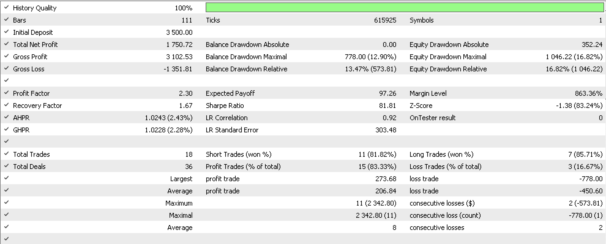
For a ‘case study’ we run tests on GBPUSD from the start of this year to the first of June. This gives us the report below:

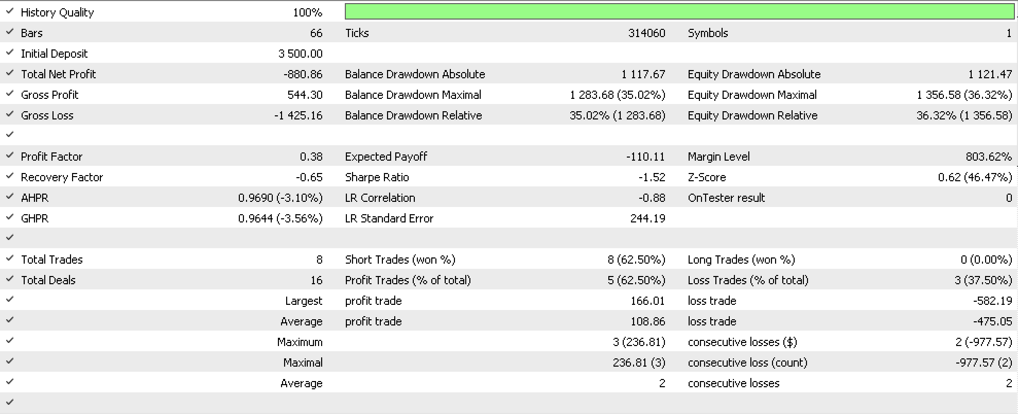
On walking forward up to August we get negative results that are in the below report:

The forecast accuracy based on the walk forward report seems to be in question which could be due to an incomplete optimization run (was run for first 3 generations only), or too small a test window since we looked at only three years and dependable systems require longer periods. The source code is attached so this could be addressed by the reader. What is demonstrated here though, as with all articles in the series, is potential for developing trade systems.

Conclusion

In conclusion, in everyday life quite often our database tables or formats of storing data are bound to grow not just in size, but also in complexity. This last point has been demonstrated here by looking at a dataset that gets more complex with the addition of data columns. We looked to exploit this for our purposes by considering time staggered data sets in an effort to make forecasts. While the optimization results showed potential given a run of only 3 generations, these runs were not able to walk forward. This could be remedied by pairing this signal class with another signal class or more extensive testing on longer periods may be undertaken.

On the article subject though, natural transformations are quite good at handling varied data structures not just cases when a data set is evolving due to business or analysis needs but possibly in cases where a comparison is necessary and by default the dimensions (number of columns) of both data sets is not the same. This is a feature that is certainly bound to come in handy across a few disciplines.

References

References are mostly Wikipedia as always. Please see the links within the article.

As a general note the attached signal file needs to be assembled with the MQL5 Wizard. This article can serve as an orientation if anyone is unfamiliar with the wizard classes.