MQL5 Wizard techniques you should know (Part 04): Linear Discriminant Analysis

Linear discriminant analysis (LDA) is a very common dimensionality reduction technique for classification problems. Like kohonen maps in prior article if you have high-dimensional data (i.e. with a large number of attributes or variables) from which you wish to classify observations, LDA will help you transform your data so as to make the classes as distinct as possible. More rigorously, LDA will find the linear projection of your data into a lower-dimensional subspace that optimizes some measure of class separation. The dimension of this subspace is never more than the number of classes. For this article we will look at how LDA can be used as a signal, trailing indicator and money management tool. But first let’s look at an intrepid definition then work our way to its applications. 

LDA is very much like the techniques PCA, QDA, & ANOVA; and the fact that they are all usually abbreviated is not very helpful. This article isn’t going to introduce or explain these various techniques, but simply highlight their differences.

1) Principal components analysis (PCA):

LDA is very similar to PCA: in fact, some have asked whether or not it would make sense to perform PCA followed by LDA regularisation ( to avoid curve fitting). That is a lengthy topic which perhaps should be an article for another day.

For this article though, crucial difference between the two dimensionality reduction methods is PCA tries to find the axes with maximum variance for the whole data set with the assumption being the more dispersed the data the more the separability, whereas LDA tries to find the axes that actually set the data apart based on  classification.

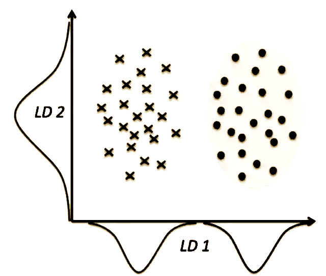
So from the illustration above, it’s not hard to see that PCA would give us LD2, whereas LDA would give us LD1. This makes the main difference (and therefore LDA preference) between PCA and LDA painfully obvious: just because a feature has a high variance (dispersion), doesn’t mean it will be useful in making predictions for the classes.

2) Quadratic discriminant analysis (QDA):

QDA is a generalization of LDA as a classifer. LDA assumes that the class conditional distributions are Gaussian with the same covariance matrix, if we want it to do any classification for us.

QDA doesn’t make this homoskedasticity assumption, and attempts to estimate the covariance of all classes. While this might seem like a more robust algorithm (given fewer assumptions), it also implies there is a much larger number of parameters to estimate. It is well established that the number of parameters grows quadratically with the number of classes! So unless you can guarantee that your covariance estimates are reliable, you might not want to use QDA.

After all of this, there might be some confusion about the relationship between LDA, QDA, such as what’s better suited for dimensionality reduction, and what is better at classification, etc. This CrossValidated post and everything that it links to, could help.

3) Analysis of variance (ANOVA):

LDA and ANOVA seem to have similar aims: both try to break-down an observed variable into several independent/dependent variables. However, the instrument used by ANOVA as per Wikipedia, is the   mirrored version of what LDA uses:

"LDA is closely related to analysis of variance (ANOVA) and regression analysis, which also attempt to express one dependent variable as a linear combination of other features or measurements. However, ANOVA uses  categorical independent variables and a  continuous dependent variable, whereas discriminant analysis has  continuous independent variables and a  categorical dependent variable (i.e. the class label)."

 

LDA is typically defined as follows.

Let:

• n  be the number of classes
• μ  be the mean of all observations
• N i  be the number of observations in the i th class
• μ i  be the mean of the  i th class
• Σ i  be the scatter matrix of the  i th class

Now, define  SW to be the within-class scatter matrix, given by

SW = ∑ i = 1 n Σ i

and define  SB to be the between-class scatter matrix, given by

SB = ∑ i = 1 n N i ( μ i − μ ) ( μ i − μ ) T

Diagonalize  SW − 1 SB to get its eigenvalues and eigenvectors.

Pick the  k  largest eigenvalues, and their associated eigenvectors. We will project our observations onto the subspace spanned by these vectors.

Concretely, what this means is that we form the matrix  A , whose columns are the  k  eigenvectors chosen above. The CLDA class in the alglib library does exactly this and sorts the vectors based on their eigen values in descending order meaning we only need to pick the best predictor vector to make a forecast.

Like in previous articles we will use the MQL code library in implementing LDA for our expert advisor. Specifically, we will rely on the ‘CLDA’ class in the ‘dataanalysis.mqh’ file.

We will explore LDA for the forex pair USDJPY over the this year 2022 on the daily timeframe. The choice of input data for our expert is largely up to the user. In our case for this LDA the input data has a variable and class component. We need to prepare this data before running tests on it. Since we’ll be dealing with close prices, it will be ‘continuized’ by default (in its raw state). We’ll apply normalization and discretization to the variable and class components of our data. Normalization means all data is between a set minimum and maximum while discretization implies data is converted to Boolean (true or false). Below are the preparations we’ll have for 5 sets of data for our signal: -

1. Discretized variables data tracking close price changes to match class categories.
2. Normalized variables data of  raw close price changes to the range -1.0 to +1.0.
3. Continuized variables data in raw close price changes. 
4. Raw close prices.

Normalization will provide the change in close price as a proportion of the last 2 bar range in decimal (from -1.0 to +1.0), while Discretization will state whether the price rose (giving an index of 2) or remained in a neutral range (meaning index is 1) or declined (implying index of 0). We will test all data types to examine performance. This preparation is done by the 'Data' method shown below. All 4 data types are regularised with the 'm_signal_regulizer' input to define a neutral zone for our data and thus reduce white noise.

//+------------------------------------------------------------------+
//| Data Set method                                                  |
//| INPUT PARAMETERS                                                 |
//|     Index   -   int, read index within price buffer.             |
//|                                                                  |
//|     Variables                                                    |
//|             -   whether data component is variables or .         |
//|                  classifier.                                     |
//| OUTPUT                                                           |
//|     double  -   Data depending on data set type                  |
//|                                                                  |
//| DATA SET TYPES                                                   |
//| 1. Discretized variables. - 0                                    |
//|                                                                  |
//| 2. Normalized variables. - 1                                     |
//|                                                                  |
//| 3. Continuized variables. - 2                                    |
//|                                                                  |
//| 4. Raw data variables. - 3                                       |
//|                                                                  |
//+------------------------------------------------------------------+
double CSignalDA::Data(int Index,bool Variables=true)
   {
      m_close.Refresh(-1);
         
      m_low.Refresh(-1);
      m_high.Refresh(-1);
            
      if(Variables)
      {
         if(m_signal_type==0)
         {
            return(fabs(Close(StartIndex()+Index)-Close(StartIndex()+Index+1))<m_signal_regulizer*Range(Index)?1.0:((Close(StartIndex()+Index)>Close(StartIndex()+Index+1))?2.0:0.0));
         }
         else if(m_signal_type==1)
         {
            if(fabs(Close(StartIndex()+Index)-Close(StartIndex()+Index+1))<m_signal_regulizer*Range(Index))
            {
               return(0.0);
            }
            return((Close(StartIndex()+Index)-Close(StartIndex()+Index+1))/fmax(m_symbol.Point(),fmax(High(StartIndex()+Index),High(StartIndex()+Index+1))-fmin(Low(StartIndex()+Index),Low(StartIndex()+Index+1))));
         }
         else if(m_signal_type==2)
         {
            if(fabs(Close(StartIndex()+Index)-Close(StartIndex()+Index+1))<m_signal_regulizer*Range(Index))
            {
               return(0.0);
            }
            return(Close(StartIndex()+Index)-Close(StartIndex()+Index+1));
         }
         else if(m_signal_type==3)
         {
            if(fabs(Close(StartIndex()+Index)-Close(StartIndex()+Index+1))<m_signal_regulizer*Range(Index))
            {
               return(Close(StartIndex()+Index+1));
            }
            return(Close(StartIndex()+Index));
         }
      }
      
      return(fabs(Close(StartIndex()+Index)-Close(StartIndex()+Index+1))<m_signal_regulizer*Range(Index)?1.0:((Close(StartIndex()+Index)>Close(StartIndex()+Index+1))?2.0:0.0));
   }

We are using a dimensionality of four meaning each indicator value will provide 4 variables. So, for brevity in our case we will look at the last four indicator values for each data set in training. Our classification will also be basic taking on just the two classes (the minimum) in the class component of each data set. We will also need to set the number of data points in our training sample. This value is stored by input parameter ‘m_signal_points’.

LDA’s output is typically a matrix of coefficients. These coefficients are sorted in vectors and a dot product of any one of those vectors with the current indicator data point should yield a value that is then compared to similar values yielded by products of the training data set in order to classify this new/ current data point. So, for simplicity, if our training set had only 2 data points with LDA projections 0 and 1 and our new value yields a dot product of 0.9, we would conclude it is in the same category with the data point whose LDA projection was 1 since it closer to it. If on the other hand it yielded a value of say 0.1 then we would be of the opinion this new data point must belong to the same category as the data point whose LDA projection was 0. 

Training datasets are seldom only two data points therefore, in practice we would take the ‘centroid’ of each class as a comparison to the output of the new data point’s dot product to LDA’s output vector. This ‘centroid’ would be the LDA projection mean of each class.

To classify each data point as bullish or bearish, we’ll simply look at the close price change after the indicator value. If it is positive that data point is bullish, if negative it is bearish. Note it could be flat. For simplicity we’ll take flats or no price changes as also bullish as well.

The ‘ExpertSignal’ class typically relies on normalized integer values (0-100) to weight long and short decisions. Since LDA projections are bound to be double type we will normalize them as shown below to fall in the range of -1.0 to +1.0 (negative for bearish and positive for bullish). 

         // best eigen vector is the first 
         for(int v=0;v<__S_VARS;v++){ _unknown_centroid+= (_w[0][v]*_z[0][v]); }
         
         //

         
         if(fabs(_centroids[__S_BULLISH]-_unknown_centroid)<fabs(_centroids[__S_BEARISH]-_unknown_centroid) && fabs(_centroids[__S_BULLISH]-_unknown_centroid)<fabs(_centroids[__S_WHIPSAW]-_unknown_centroid))
         {
            _da=(1.0-(fabs(_centroids[__S_BULLISH]-_unknown_centroid)/(fabs(_centroids[__S_BULLISH]-_unknown_centroid)+fabs(_centroids[__S_WHIPSAW]-_unknown_centroid)+fabs(_centroids[__S_BEARISH]-_unknown_centroid))));
         }
         else if(fabs(_centroids[__S_BEARISH]-_unknown_centroid)<fabs(_centroids[__S_BULLISH]-_unknown_centroid) && fabs(_centroids[__S_BEARISH]-_unknown_centroid)<fabs(_centroids[__S_WHIPSAW]-_unknown_centroid))
         {
            _da=-1.0*(1.0-(fabs(_centroids[__S_BEARISH]-_unknown_centroid)/(fabs(_centroids[__S_BULLISH]-_unknown_centroid)+fabs(_centroids[__S_WHIPSAW]-_unknown_centroid)+fabs(_centroids[__S_BEARISH]-_unknown_centroid))));
         }

This value then is easily normalized to the typical integer (0-100) that is expected by the signal class.

   if(_da>0.0)
     {
      result=int(round(100.0*_da));
     }

 for the Check long function and,

   if(_da<0.0)
     {
      result=int(round(-100.0*_da));
     }

for the check short.

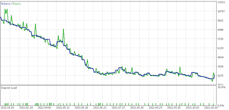
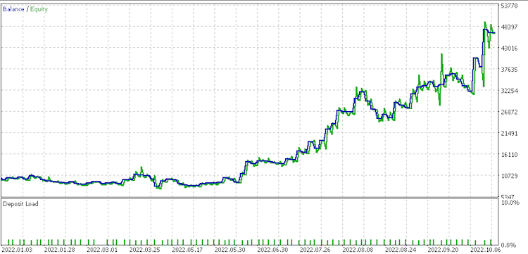
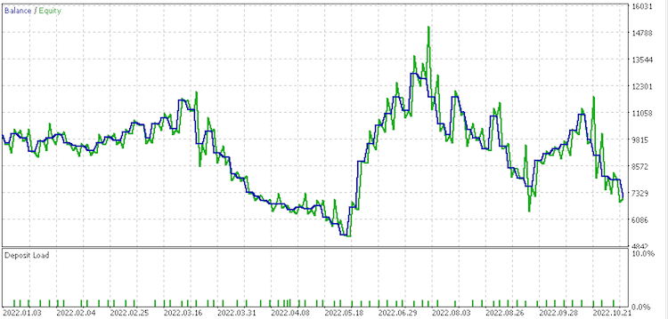
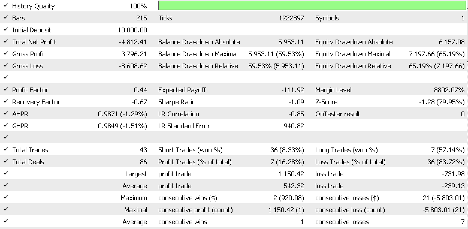
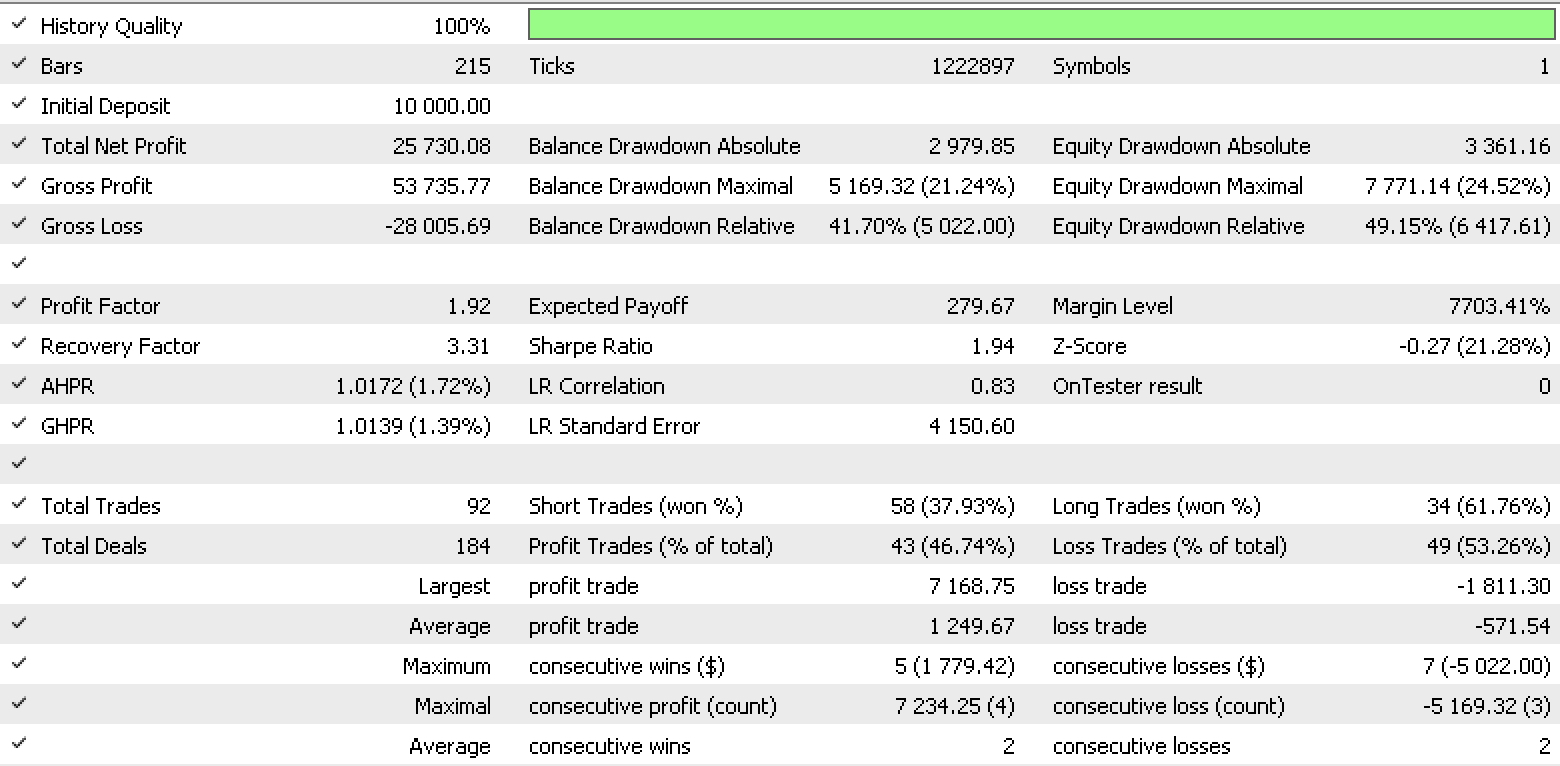
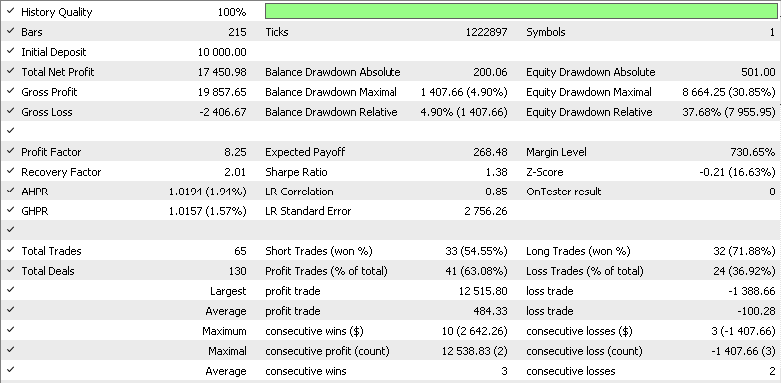
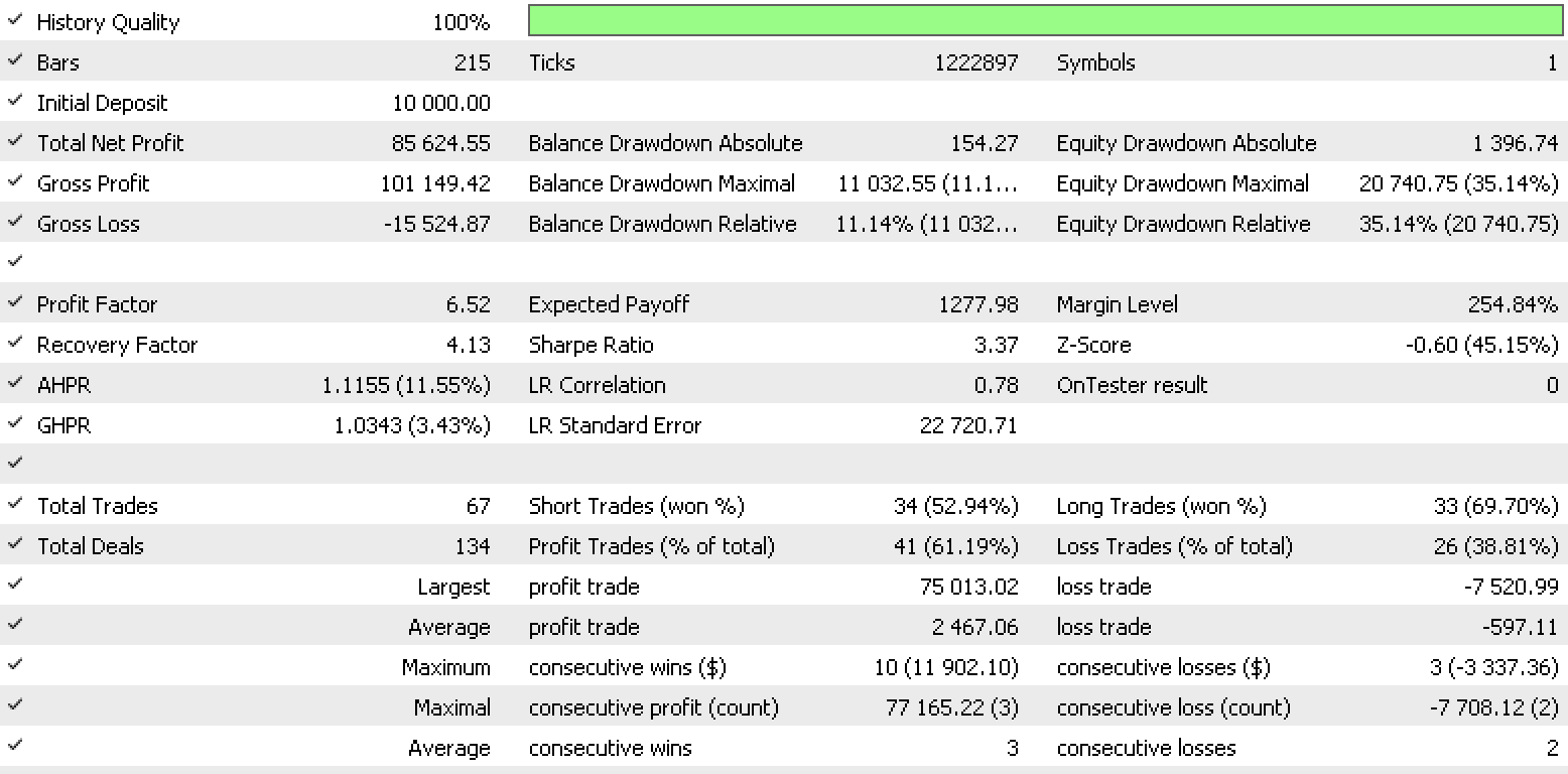
So, a test run for each of the input data types gives the strategy tester reports below.

Data set 1 report

 

Data set 2 report

 

Data set 3 report

 

Data set 4 report

  

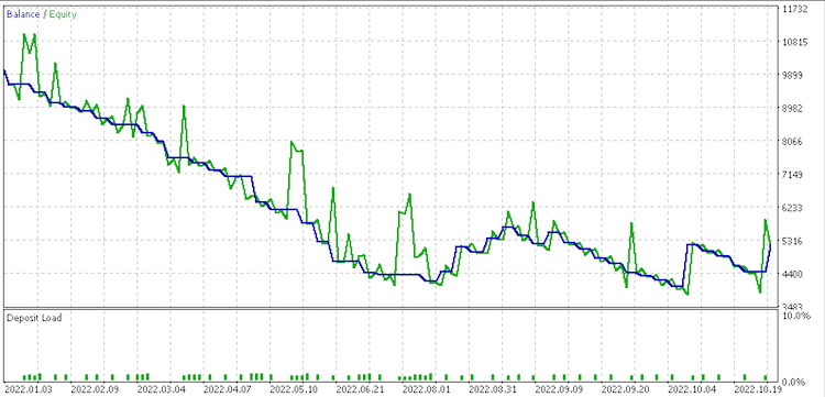
These reports exhibit the potential of LDA as tool for a trader. 

The ‘ExpertTrailing’ class adjusts or sets a stop loss for an open position. The key output here is a double for the new stop loss. So, depending on the open position we’ll consider High prices and Low prices as our primary data sets. These will be prepared as follows for both High prices and Low prices with the choice depending on the type of open position: - 

1. Discretized variables data tracking (high or low) price changes to match class categories.
2. Normalized variables data of raw (high or low) price changes to the range -1.0 to +1.0. 
3. Continuized variables data in raw (high or low) price changes. 
4. Raw (high or low) prices.

The output from the LDA will be a normalized double as with the signal class. Since this is not helpful in defining a stop loss it will be adjusted as shown below depending on the type of open position to come up with a stop loss price.

      int _index   =StartIndex();
      double _min_l=Low(_index),_max_l=Low(_index),_min_h=High(_index),_max_h=High(_index);
      
      for(int d=_index;d<m_trailing_points+_index;d++)
      {
         _min_l=fmin(_min_l,Low(d));
         _max_l=fmax(_max_l,Low(d));
         _min_h=fmin(_min_h,High(d));
         _max_h=fmax(_max_h,High(d));
      }
      
      if(Type==POSITION_TYPE_BUY)
      {
         _da*=(_max_l-_min_l);
         _da+=_min_l;
      }
      else if(Type==POSITION_TYPE_SELL)
      {
         _da*=(_max_h-_min_h);
         _da+=_max_h;
      }

Also here is how we adjust and set our new stop loss levels. For the long positions:

   m_long_sl=ProcessDA(StartIndex(),POSITION_TYPE_BUY);

   double level =NormalizeDouble(m_symbol.Bid()-m_symbol.StopsLevel()*m_symbol.Point(),m_symbol.Digits());
   double new_sl=NormalizeDouble(m_long_sl,m_symbol.Digits());
   double pos_sl=position.StopLoss();
   double base  =(pos_sl==0.0) ? position.PriceOpen() : pos_sl;
//---
   sl=EMPTY_VALUE;
   tp=EMPTY_VALUE;
   if(new_sl>base && new_sl<level)
      sl=new_sl;

What we're doing here is determining the likely low price point, until the next bar, for a long open position ('m_long_sl') and then setting it as our new stop loss if it is more than either the position's open price or its current stop loss while being below the bid price minus stops level. The data type used in calculating this is low prices.

The setting of stop loss for short positions is a mirrored version of this.

So, a test run for each of the input data type while using the … data type for signal gives the strategy tester reports below.

Data set 1 report

 

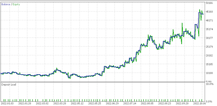
Data set 2 report

 

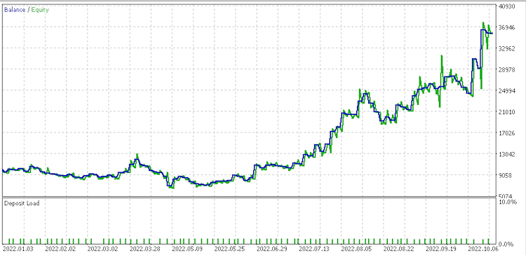
Data set 3 report

 

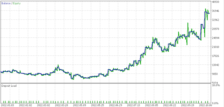
Data set 4 report.

 

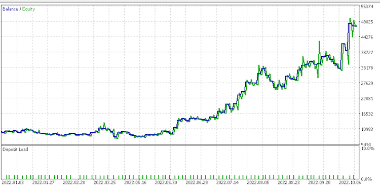
These reports perhaps point to .data set of continued raw changes as best suited given its recovery factor of 6.82.

The ‘ExpertMoney’ class sets our position lot size. This can be a function of past performance which is why we’re building on the ‘OptimizedVolume’ class. However, LDA can help with initial sizing if we consider volatility or the range between High and Low prices. Our primary data set therefore will be price bar range. We’ll look to see if price bar range is increasing or decreasing. With that let’s have the following data preparations: - 

1. Discretized variables data tracking range value changes to match class categories.
2. Normalized variables data of raw range value changes to the range -1.0 to +1.0. 
3. Continuized variables data in raw range value changes. 
4. Raw range values.

The output from the LDA will be a normalized double as with the signal and trailing class. Since once again this is not immediately helpful we'll make adjustments shown below to better project a new bar range.

      int _index   =StartIndex();
      double _min_l=Low(_index),_max_h=High(_index);
      
      for(int d=_index;d<m_money_points+_index;d++)
      {
         _min_l=fmin(_min_l,Low(d));
         _max_h=fmax(_max_h,High(d));
      }
   
      _da*=(_max_h-_min_l);
      _da+=(_max_h-_min_l);

The setting of open volume is handled by 2 mirrored functions depending on whether the expert is opening a long or short position. Below are highlights for a long position.

   double _da=ProcessDA(StartIndex());
   
   if(m_symbol==NULL)
      return(0.0);
   
   sl=m_symbol.Bid()-_da;
   
//--- select lot size
   double _da_1_lot_loss=(_da/m_symbol.TickSize())*m_symbol.TickValue();
   double lot=((m_percent/100.0)*m_account.FreeMargin())/_da_1_lot_loss;
   
//--- calculate margin requirements for 1 lot
   if(m_account.FreeMarginCheck(m_symbol.Name(),ORDER_TYPE_BUY,lot,m_symbol.Ask())<0.0)
     {
      printf(__FUNCSIG__" insufficient margin for sl lot! ");
      lot=m_account.MaxLotCheck(m_symbol.Name(),ORDER_TYPE_BUY,m_symbol.Ask(),m_percent);
     }
   
//--- return trading volume
   return(Optimize(lot));

What is noteworthy here is we determine projected change in range price and subtract this projection from our bid price (Should have subtracted stops level as well). This will give us a 'risk adjusted' stop loss from which if we use the percent input parameter as a maximum risk loss parameter, we can compute a lot size that will cap our drawdown percentage at the percent input parameter value should we experience a drawdown below the bid price which is as projected.

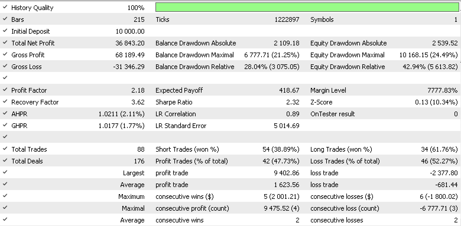
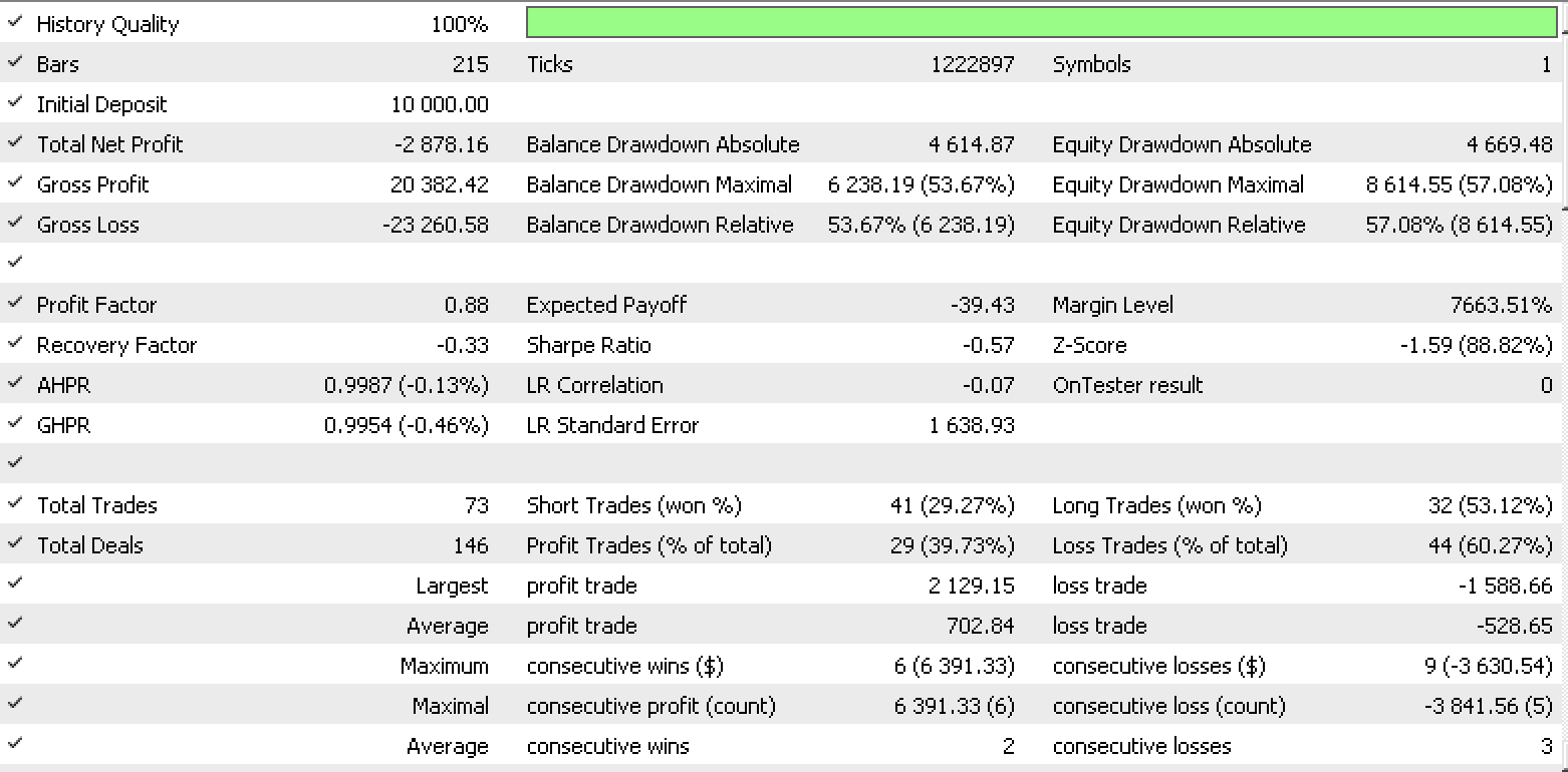
So, a test run for each of the input data type while using the raw close prices data type for signal and … for trailing gives the strategy tester reports below.

Data set 1 report

 

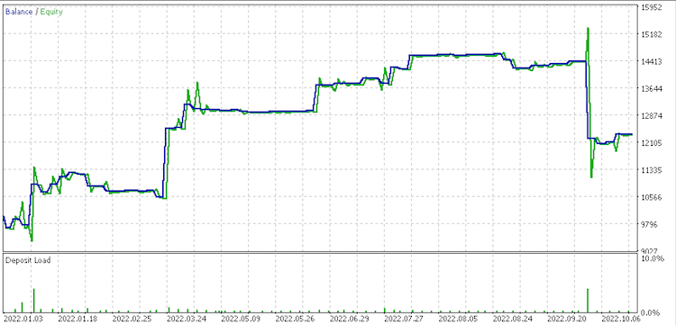
Data set 2 report

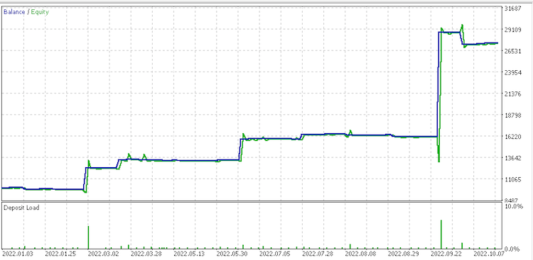
Data set 3 report

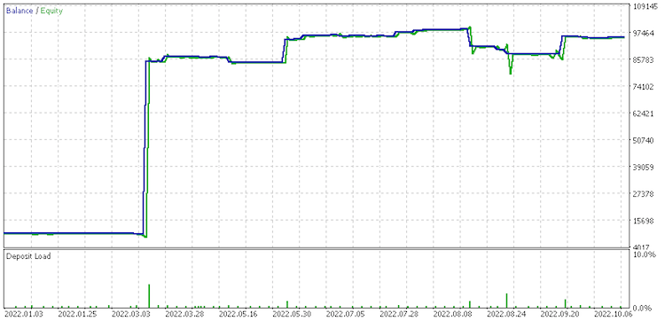
Data set 4 report

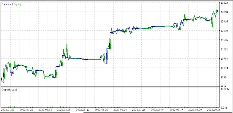
It appears data set of discrete range value changes is most promising for money management. Noteworthy as well is the huge variance in results for the data sets at money management considering they are all using the same signal and trailing settings.

This article has highlighted potential of discriminant analysis’ use as a trading tool in an expert advisor. It was not exhaustive. Further analysis could be undertaken with more diverse data sets that span longer periods.