Category Theory in MQL5 (Part 18): Naturality Square

Introduction

Category theory’s bearing in MQL5 for trader’s is bound to be subjective and this far in these series we have used its systems-wide approach in emphasizing morphisms over objects to make forecasts and classifications on financial data.

Natural transformations, a crux concept in category theory, is often taken as simply a mapping between functors. This pedestrian view, though not wrong, can lead to some confusion if you consider that a functor is linking two objects, because the question becomes which objects does a natural transformation link? Well the short answer is the two codomain objects of the functors and for this article we will try to show a buildup leading to this definition and also include an instance of the expert trailing class that uses this morphism to forecast changes in volatility.

The categories to be used as examples in illustrating natural transformations will be two, which is the minimum number for a pair of functors used to define a natural transformation. The first will consist of two objects that comprise of normalized indicator values. The indicators we will consider are ATR and Bollinger Bands values. The second category, which will serve as the codomain category since the two functors will be leading to it, will include four objects that will capture price bar ranges of the values we want to forecast.

Understanding the Categories

The indicator values category is mentioned in our article only to help in understanding the concepts being outlined here. In the end it plays a minimal to no role in forecasting the volatility we’re interested in because we will primarily be relying on the naturality square to accomplish this. It is foundational none the less. There is not a lot of definitive information on the naturality square available online but this post could be interesting reading for those looking for more resources on the subject outside of what is shared here.

So back to our domain category and as mentioned it has two objects, one with ATR values and the other with Bollinger Bands values. These values are normalized such that the objects have a fixed cardinality (size). The values represented in each object are respective changes to indicator values. These changes are logged in steps of 10% from minus 100% to plus 100% meaning each object’s cardinality is 21. They therefore comprise the following values:

{

-100, -90, -80, -70, -60, -50, -40, -30, -20, -10,

 0,

 10, 20, 30, 40, 50, 60, 70, 80, 90, 100

}

The morphism linking these element identical objects will pair values based on whether they were registered at the same time thus providing a current log of changes in the two indicator values.

These indicator-change-values could have been from any other volatility related indicator. The principles remain the same. The change in the indicator value is divided by the sum of the absolute values of the previous and current indicator reading to get a decimal fraction. This fraction is then multiplied by 10 and rounded off to no decimal place. It is then multiplied by 10 again and assigned an index in our objects outlined above depending on the value it is equivalent to.

The price bar ranges category will comprise four objects that will be the main focus of the naturality square we’ll use in making projections. Since our domain category (with indicator changes) consists of two objects, and we have two functors leading from it to this codomain, it follows each of these functors is mapping to an object. The objects mapped to do not always have to be distinct, however in our case in order to help clarify our concepts, we are letting each object mapped from in the domain category have its own codomain object in the price ranges category. Thus 2 objects times 2 functors will yield 4 end point objects, the members of our codomain category.

Since we have four objects and do not want to have duplicity, each object will log a different set of price bar range changes. To assist in this the two functors will represent different forecast deltas. One functor will map the price bar range after one bar while the other functor will map the price range changes after two bars. In addition, the mappings from the ATR object will be for price ranges across a single bar while those from the Bollinger Bands object will be for price ranges across two bars. This can be summarized by the listing below which implements this:

      CElement<string> _e;
      for(int i=0;i<m_extra_training+1;i++)
      {
         double _a=((m_high.GetData(i+_x)-m_low.GetData(i+_x))-(m_high.GetData(i+_x+1)-m_low.GetData(i+_x+1)))/((m_high.GetData(i+_x)-m_low.GetData(i+_x))+(m_high.GetData(i+_x+1)-m_low.GetData(i+_x+1)));
         double _c=((m_high.GetData(i+_x)-m_low.GetData(i+_x))-(m_high.GetData(i+_x+2)-m_low.GetData(i+_x+2)))/((m_high.GetData(i+_x)-m_low.GetData(i+_x))+(m_high.GetData(i+_x+2)-m_low.GetData(i+_x+2)));
         double _b=((fmax(m_high.GetData(i+_x),m_high.GetData(i+_x+1))-fmin(m_low.GetData(i+_x),m_low.GetData(i+_x+1)))
                     -(fmax(m_high.GetData(i+_x+2),m_high.GetData(i+_x+3))-fmin(m_low.GetData(i+_x+2),m_low.GetData(i+_x+3))))
                     /((fmax(m_high.GetData(i+_x),m_high.GetData(i+_x+1))-fmin(m_low.GetData(i+_x),m_low.GetData(i+_x+1)))
                     +(fmax(m_high.GetData(i+_x+2),m_high.GetData(i+_x+3))-fmin(m_low.GetData(i+_x+2),m_low.GetData(i+_x+3))));
         double _d=((fmax(m_high.GetData(i+_x),m_high.GetData(i+_x+1))-fmin(m_low.GetData(i+_x),m_low.GetData(i+_x+1)))
                     -(fmax(m_high.GetData(i+_x+3),m_high.GetData(i+_x+4))-fmin(m_low.GetData(i+_x+3),m_low.GetData(i+_x+4))))
                     /((fmax(m_high.GetData(i+_x),m_high.GetData(i+_x+1))-fmin(m_low.GetData(i+_x),m_low.GetData(i+_x+1)))
                     +(fmax(m_high.GetData(i+_x+3),m_high.GetData(i+_x+4))-fmin(m_low.GetData(i+_x+3),m_low.GetData(i+_x+4))));
         
         ...
      }

These objects will be single sized as they only log the current change. The morphisms amongst them will flow in a square commute from the single bar price range projection to the two-bar price range forecast, two price bars ahead. More on this is shared when we formally define natural transformations below.

The relationship between price bar ranges and the sourced market data is also shown in our source above. The changes logged in each object are not normalized as was the case with the indicator values, but rather the changes in the range are divided by the sum of the current and prior bar ranges to produce an unrounded decimal value.

Functors: Linking Indicator Values to Price Bar Ranges

Functors were introduced to our series four articles back but they are being looked at here as a pair on two categories. Recall functors do not map just objects but they also map morphisms so keeping with that, since our domain category of indicator values has two objects and a morphism this implies there will be three output points in our codomain category, two from an object and one from a morphism for each functor. With two functors this makes six end points in our codomain.

The mapping of the normalized indicator integer values to decimal price bar range changes, changes that are logged as fractions and not the raw values, could be accomplished with the help multi-layer perceptrons as we have explored in the last two articles. There is still a host of other methods of doing this mapping unexplored yet in these series, such as the random forest for instance.

This illustration here is only for completeness. To properly show what a natural transformation is and all its prerequisites. As traders when faced with new concepts the critical question is always what is its application and benefit? That’s why I stated at the onset that for our forecasting purposes our focus will be the naturality square that is solely determined by the four objects in the codomain category. So, the mention of the domain category and its objects here is simply helping with defining natural transformations and it is not helping with our specific application for this article.

Natural Transformations: Bridging the Gap

With that clarified can now look at the natural transformation axioms so as to move on to the applications.Formally, a natural transformation between functors

F: C --> D

and

G: C --> D

is a family of morphisms

ηA: F(A) --> G(A)

for all objects A in category C such that for all morphisms

f: A --> B

in category C, the following diagram commutes:

 

There is a healthy amount of material on natural transformations online but none the less it may be helpful to look at a more illustrative definition leads up to the naturality square. To that end let’s suppose you have two categories C & D with category C having two objects X and Y defined as follows:

X = {5, 6, 7}

and

Y = {Q, R, S}

Let’s also suppose we have a morphism between these objects, f defined as:

f: X à Y

such that f(5) = S, f(6) = R, and f(7) = R.

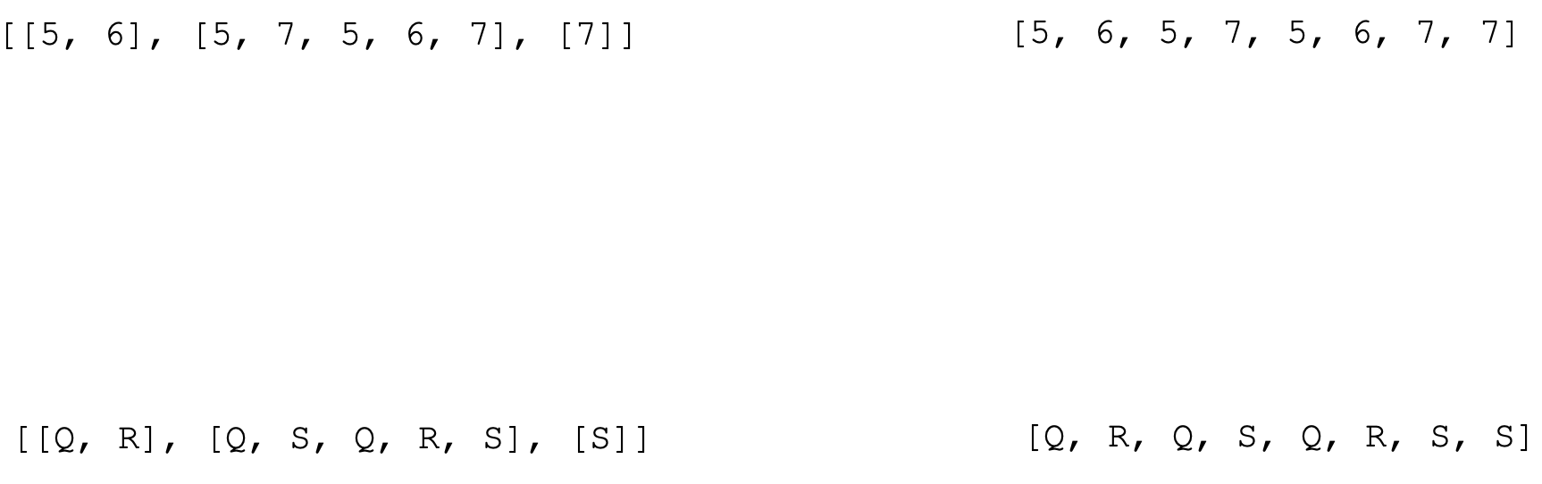
For this example, the two functors F and G, between the categories C and D that will do two simple things. Prepare a list and a list of lists respectively. So functor F when applied to X would output:

[5, 6, 5, 7, 5, 6, 7, 7]

and similarly, the functor G (list of lists) would give:

[[5, 6], [5, 7, 5, 6, 7], [7]]

If we apply these functors similarly to object Y we would end up with 4 objects in the codomain category D. These are represented as shown below:

Notice we are now focusing on only four objects in category D. Since we have two objects in our domain category C, we are also going to have two natural transformations each with respect to an object in C. These are represented as below:

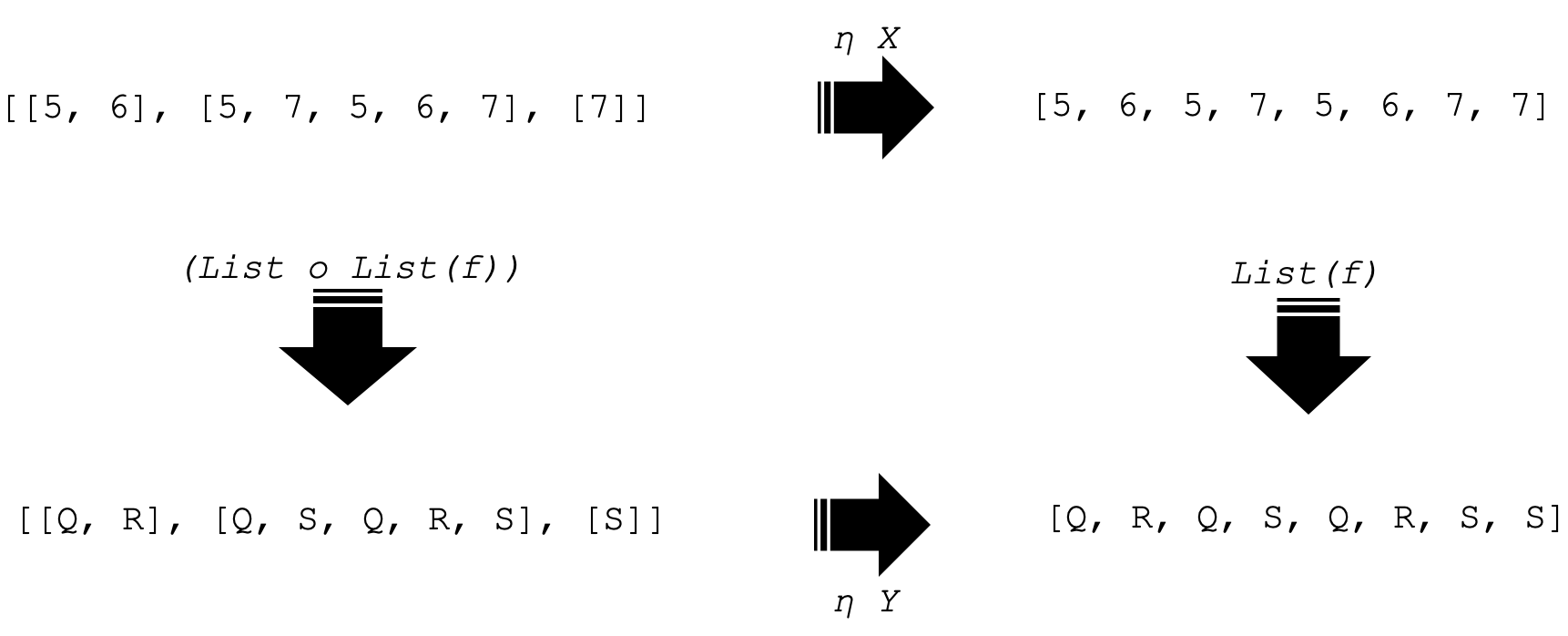
The representation above is the square of naturality. And it commutes as you can see from the arrows indicated. So, the two horizontal arrows are our natural transformations (NTs) with respect to each object in C and the vertical arrows are functor outputs when applied to the morphism f in category C for the functors F and G.

The importance of preserving structure and relationships is a key aspect of NTs that could be overlooked and yet even though it is so simple, it is crucial. To make our point let’s consider an example in the culinary/ cuisine field. Supposing two famous chefs let’s call them A and B each have a unique way preparing the same dish from a standard set of ingredients. We would take the ingredients to be an object in a broader category of ingredient types and the two dishes each chef produces would belong to also another broader category of dish types. Now a natural transformation between the two dishes produced by our chefs A and B would log the ingredients, and extra cooking preparations required to modify the dish produced by chef A to that produced by chef B. With this approach we are logging more information and can in fact check and see if say a chef C’s dish would also need such a similar NT to match chef B’s dish or if not by what degree? But besides comparison the NT’s application to get chef B’s dish would require chef A’s recipe, cooking styles and methods. Meaning they are preserved and respected. This preservation is important for records but also can be a means of developing new recipes or even checking existing ones based on somebody’s dietary restrictions.

Applications: Forecasting Volatility

With that we can now look at possible applications in forecasting. Projecting the next change in price bar range is something we have considered a lot in these series and therefore preliminary explanations may not be quaint. But to recap we use this forecast to determine firstly if we need to adjust the trailing stop on open positions, and secondly by how much we need to adjust it.

The implementation of the naturality square as a key tool in this will be with the help of multi-layer perceptrons (MLPs) as was the case in our last two articles with the difference here being these MLPs are composed around a square commutation. This allows us to check our forecasts since any two legs could produce a projection. The four corners of the square reflect different forecasts at some point in the future of changes in the range of our price bars. As we move towards corner D the more we look into the future with corner A projecting the range change for just the next bar. This means if we are able to train MLPs that link up all four corners, using the range change for the most recent price bar, we can make projections much further ahead beyond just a single bar.

The steps involved in applying our NTs to get a forecast are highlighted by the listing below:

//+------------------------------------------------------------------+
//| NATURAL TRANSFORMATION CLASS                                     |
//+------------------------------------------------------------------+
class CTransformation
   {
      protected:
      
      public:
      
      CDomain<string>               domain;  //codomain object of first functor
      CDomain<string>               codomain;//codomain object of second functor
      
      uint                          hidden_size;
      CMultilayerPerceptron         transformer;
      CMLPBase                      init;
      
      void                          Transform(CDomain<string> &D,CDomain<string> &C)
                                    {
                                       domain=D;
                                       codomain=C;
                                       
                                       int _inputs=D.Cardinality(),_outputs=C.Cardinality();
                                       
                                       if(_inputs>0 && _outputs>0)
                                       {
                                          init.MLPCreate1(_inputs,hidden_size+fmax(_inputs,_outputs),_outputs,transformer);
                                       }
                                    }
      
      //
      void                          Let()
                                    {
                                       this.codomain.Let();
                                       this.domain.Let();
                                    };
      
                                    CTransformation(void){ hidden_size=1; };
                                    ~CTransformation(void){};
   };

First off, we have our NT class listed above. And as from the casual definition you would expect it to include instance of the two functor’s it is linking but that though applicable, was not succinct enough. What is key with NTs is the two domains mapped to by the functors and these are what is highlighted.

//+------------------------------------------------------------------+
//| NATURALITY CLASS                                                 |
//+------------------------------------------------------------------+
class CNaturalitySquare
   {
      protected:
      
      public:
      
      CDomain<string>               A,B,C,D;
      
      CTransformation               AB;
      
      uint                          hidden_size_bd;
      CMultilayerPerceptron         BD;
      
      uint                          hidden_size_ac;
      CMultilayerPerceptron         AC;
      
      CTransformation               CD;
      
      CMLPBase                      init;
      
      
                                    CNaturalitySquare(void){};
                                    ~CNaturalitySquare(void){};
   };

The naturality square, whose diagram is shown above, would also have its class represented as shown with instances of the NT class. Its four corners expressed by A, B, C, and D, are objects captured by the domain class and only two of its morphisms would be direct MLPs as the other two a recognized as NTs.

Practical Implementation in MQL5

Practical implementation in MQL5 given our use of MLPs is bound to face challenges primarily in how we train and store what we have learnt (network weights). For this article, unlike the last two, weights from training are not stored at all meaning on each new bar a new instance of each of the four MLPs is generated and trained. This is implemented with the refresh function as shown below:

//+------------------------------------------------------------------+
//| Refresh function for naturality square.                          |
//+------------------------------------------------------------------+
double CTrailingCT::Refresh()
   {
      double _refresh=0.0;
      
      m_high.Refresh(-1);
      m_low.Refresh(-1);
      
      int _x=StartIndex();
      
      // atr domains capture 1 bar ranges       
      // bands' domains capture 2 bar ranges    
      // 1 functors capture ranges after 1 bar  
      // 2 functors capture ranges after 2 bars 
      
      int _info_ab=0,_info_bd=0,_info_ac=0,_info_cd=0;
      CMLPReport _report_ab,_report_bd,_report_ac,_report_cd;
      CMatrixDouble _xy_ab;_xy_ab.Resize(m_extra_training+1,1+1);
      CMatrixDouble _xy_bd;_xy_bd.Resize(m_extra_training+1,1+1);
      CMatrixDouble _xy_ac;_xy_ac.Resize(m_extra_training+1,1+1);
      CMatrixDouble _xy_cd;_xy_cd.Resize(m_extra_training+1,1+1);
      
      CElement<string> _e;
      for(int i=0;i<m_extra_training+1;i++)
      {
         ...
         
         if(i<m_extra_training+1)
         {
            _xy_ab[i].Set(0,_a);//in
            _xy_ab[i].Set(1,_b);//out
            
            _xy_bd[i].Set(0,_b);//in
            _xy_bd[i].Set(1,_d);//out
            
            _xy_ac[i].Set(0,_a);//in
            _xy_ac[i].Set(1,_c);//out
            
            _xy_cd[i].Set(0,_c);//in
            _xy_cd[i].Set(1,_d);//out
         }
      }
      
      m_train.MLPTrainLM(m_naturality_square.AB.transformer,_xy_ab,m_extra_training+1,m_decay,m_restarts,_info_ab,_report_ab);
     
      ...

      //
      if(_info_ab>0 && _info_bd>0 && _info_ac>0 && _info_cd>0)
      {
         ...
      }
      
      return(_refresh);
   }

The refresh function above trains MLPs initialized with random weights on just the recent price bar. This is clearly bound to be insufficient for other trade systems or implementations of the code shared however an input parameter ‘m_extra_training’ whose default value of zero is maintained for our testing purposes, can be adjusted upwards to provide more comprehensive testing prior to making forecasts.

Use of the parameter for extra training is bound to create a performance overload on the expert and in fact points to why the reading and writing of weights from training has been avoided all together for this article.

Benefits and Limitations

If we run tests on EURUSD on the daily time frame from 2022.08.01 to 2023.08.01, one of our best runs yields the following report:

If we run tests with these same settings on a non-optimized period, in our case the one-year period prior to our testing range we get negative results that do not reflect the good performance we got in the report above. As can be seen all profits were from stop losses.

Compared to approaches we used earlier in the series, in projecting volatility, this approach is certainly a resource intensive and clearly requires modifications in the way our four objects in the naturality square are defined in order to enable forward walks over non-optimized periods.

Conclusion

To sum up here the key concepts laid out was natural transformations. They are significant in linking categories by capturing the difference between a parallel pair of functors bridging the categories. Applications explored here were for forecasting volatility by utilizing the naturality square however other possible applications do include generation of entry and exit signals and well as position sizing. In addition, it may be helpful to mention, for this article and through out these series we have not performed any forward runs on optimized settings obtained. So chances are they will not work out of the box (i.e. as the code is provided), but could once modifications are made such as by pairing these ideas with other strategies the reader may use. This is why the use of MQL5 wizard classes comes in handy because it seamlessly allows this.

References

Wikipedia and stack exchange as per shared hyperlinks.

Notes on Attachments

Do place the files 'SignalCT_16_.mqh' in the folder 'MQL5\include\Expert\Signal\' and the file 'ct_16.mqh' can be in 'MQL5\include\’ folder.

In addition, you may want to follow this guide on how to assemble an Expert Advisor using the wizard since you would need to assemble them as part of an Expert Advisor. As stated in the article I used no trailing stop and fixed margin for money management both of which are part of MQL5's library. As always, the goal of the article is not to present you with a Grail but rather an idea which you can customize to your own strategy.