
Neural networks made easy (Part 34): Fully Parameterized Quantile Function

Contents
- Introduction
- 1. Theoretical Aspects of Complete Parameterization
- 2. Implementation in MQL5
- 3. Testing
- Conclusion
- References
- Programs used in the article
Introduction
We continue studying distributed Q-learning algorithms. Earlier we have already considered two algorithms. In the first one [4], our model learned the probabilities of receiving a reward in a given range of values. In the second algorithm [5], we used a different approach to solving the problem. We trained the model to predict the reward level with a given probability.
Obviously, in both algorithms, we need some a priori knowledge about the nature of the reward distribution in order to solve the problem. In the first algorithm, we feed the expected reward levels into the model, while in the second one the user's task is a little easier. We need to input into the model a series of quantiles, the size of which is normalized in the range from 0 to 1 and which are arranged in ascending order. However, without knowing the true distribution of reward values, it is difficult to determine the number of quantiles needed and the volumes of each.
In should be noted here that we used the assumption of a uniform distribution of the studied sequence. So, we used uniform ranges of quantiles. The main regulating hyperparameter was the number of such quantiles. It is determined empirically on the validation dataset.
1. Theoretical Aspects of Complete Parameterization
Both of the mentioned methods require the preliminary study of the training dataset and the optimization of hyperparameters. At the same time, it should be noted that when optimizing hyperparameters, we choose some average values. In other words, we choose something that can get us as close as possible to the desired goal. The chosen parameters should satisfy all possible states of the system under study as much as possible. We have also made an assumption of a uniform distribution. Therefore, we actually have a model full of various compromises. Obviously, such a model will be far from optimal.
To improve the credibility and to minimize the prediction error, we have to increase the number of quantiles to be trained. This, in turn, increases the model training time and the model size. In most cases, this approach is ineffective. However, our purpose is to study of the environment as thoroughly as possible. Therefore, it would seem an appropriate approach to abandon fixed value categories in the first algorithm and fixed quantiles in the second algorithm.
1.1. Implicit Quantile Networks (IQN)
The use of quantiles looks more promising here. Because in order to determine the categories, we need to fully study the original distribution and define its limits. But the model is not prepared for values that fall outside the specified range. The category model is not universal and it varies in different tasks.
At the same time, the probabilities of event occurrences have clear limits in the range from 0 to 1. But the use of a uniform distribution of quantiles limits our freedoms and the range of optimizable functions. It would be good to find such an algorithm in which the model itself can determine the optimal quantile distribution without increasing the number of quantiles.
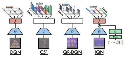
The first such algorithm was proposed in July 2018, in the article Implicit Quantile Networks for Distributional Reinforcement Learning. But the authors approached the problem of optimal quantiles in a slightly different way. They built their algorithm on the basis of QR-DQN we discussed earlier. But instead of searching for optimal quantiles, the authors decided to generate them randomly and feed them into the model along with the initial data that described the state of the environment. The idea is as follows: during the training process, the same system states with different quantile distributions will be input into the model. As a result, the model is forced to use not a specific slice of the quantile function, but its full approximation.
This approach enables the training of a model that is less sensitive to the 'number of quantiles' hyperparameter. Their random distribution allows the expansion of the range of approximated functions to non-uniformly distributed ones.
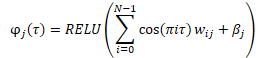
Before the data is input into the model, an embedding of randomly generated quantiles is created according to the formula below.
There are different options in combining the resulting embedding with the tensor of the original data. This can be either a simple concatenation of two tensors or a Hadamard (element-by-element) multiplication of two matrices.
Below is a comparison of the considered architectures, presented by the authors of the article.
The model effectiveness is confirmed by tests carried out on 57 Atari games. Below is a comparison table from the original article [8]
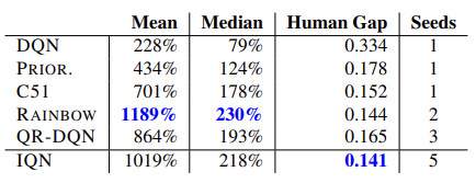
Hypothetically, given the unlimited size of the model, this approach allows learning any distribution of the predicted reward.
1.2. Fully Parameterized Quantile Function (FQF)
The presented model of implicit quantile networks is capable of approximating various functions. But this process is connected with the growth of the model. However, resources are limited in practice. When generating random quantiles, there is always a risk of obtaining non-optimal values, both when training and when using the model.
In November 2019, Fully Parameterized Quantile Function for Distributional Reinforcement Learning was proposed.
Essentially, this is the same IQN model. But instead of a random quantile generator, it uses a fully connected neural layer, which returns the distribution of quantiles based on the current state of the environment given as input. The model generates a quantile distribution for each 'state-action' value pair. This allows the approximation of the optimal distribution of the expected reward for each action in a particular system state. This is what we were talking about at the beginning of this article.
The main requirements for quantiles are still preserved. These include in the range from 0 to 1. To achieve this effect, the algorithm uses data normalization at the neural layer output. The data is normalized using the Softmax function and then cumulative (accumulative) addition of elements of the normalized vector is applied.
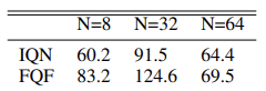
In the original article, the authors present the results of algorithm testing on 55 Atari games. Below is a summarized table of results from the original article. The presented data demonstrates the superiority of the quantile function full parametrization algorithm over other distributed Q-learning algorithms. But the cost of it is the performance of the model. The additional quantile generation model requires additional computational resources.
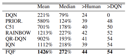
The method authors conducted experiments to select the optimal number of quantiles and suggest using a distribution of 32 quantiles.
We will study the method algorithm in more detail while implementing it in further topics.
2. Implementation in MQL5
In their article, the method authors talk about the use of two neural networks: one for generating the distribution of quantiles and the other one for approximating the quantile function. However, the described algorithm actually also uses a third convolutional network which creates an embedding of the environment state. This state embedding is the source data of the algorithm under consideration.
However, the library we created earlier is focused on building sequential models. It does not include an algorithm to pass an error gradient between models, which can be required when training multiple sequential models.
Of course, we can use the Transfer Learning mechanism and sequentially train each individual model. But I decided to implement the entire algorithm within a single model.
To create the environment state embedding we use convolutional models discussed earlier [1]. Therefore, we can easily build such a model with existing tools.
Next, we need to implement the FQF algorithm. In my opinion, the easiest way to implement it within our library concept is to create a new neural layer class. We input the embedding of the current state of the system being analyzes and the layer will output the agent action. Thus, inside the new class, we will build an agent of our model.
We will create the new class CNeuronFQF deriving it from the neural layer base class CNeuronBaseOCL. The new class will override our usual set of methods. In the protected block, we will declare the internal objects that we will use when implementing the FQF algorithm. We will learn more about the purpose of the object in the process of constructing the algorithm.
class CNeuronFQF : protected CNeuronBaseOCL
  {
protected:
   //--- Fractal Net
   CNeuronBaseOCL    cFraction;
   CNeuronSoftMaxOCL cSoftMax;
   //--- Cosine embeding
   CNeuronBaseOCL    cCosine;
   CNeuronBaseOCL    cCosineEmbeding;
   //--- Quantile Net
   CNeuronBaseOCL    cQuantile0;
   CNeuronBaseOCL    cQuantile1;
   CNeuronBaseOCL    cQuantile2;
   //---
   virtual bool      feedForward(CNeuronBaseOCL *NeuronOCL) override;
   virtual bool      updateInputWeights(CNeuronBaseOCL *NeuronOCL) override;

public:
                     CNeuronFQF();
                    ~CNeuronFQF();
   //---
   virtual bool      Init(uint numOutputs, uint myIndex, COpenCLMy *open_cl,
                          uint actions, uint quantiles, uint numInputs,
                          ENUM_OPTIMIZATION optimization_type, uint batch);
   virtual bool      calcInputGradients(CNeuronBaseOCL *NeuronOCL);
   //---
   virtual bool      Save(int const file_handle) override;
   virtual bool      Load(int const file_handle) override;
   //---
   virtual int       Type(void) override        const { return defNeuronFQF; }
   virtual CLayerDescription* GetLayerInfo(void) override;
  };
In our class, we use static internal objects, and thus the class constructor and destructor can be left empty.
The class and internal objects are initialized in the Init method. To initialize internal objects, we will need the following parameters:
- numOutputs — the number of neurons in the next layer
- myIndex — the index of the current neuron in the layer
- open_cl — a pointer to the object for working with the OpenCL device
- actions — the number of possible agent actions
- quantiles — the number of quantiles
- numInputs — the size of the previous neural layer
- optimization_type — function used to optimize the model parameters
- batch — parameter update batch size
bool CNeuronFQF::Init(uint numOutputs, uint myIndex, COpenCLMy *open_cl,

                      uint actions, uint quantiles, uint numInputs,
                      ENUM_OPTIMIZATION optimization_type, uint batch)
  {
   if(!CNeuronBaseOCL::Init(numOutputs, myIndex, open_cl, actions, optimization, batch))
      return false;
   SetActivationFunction(None);
In the method body, we do not define a block for checking the received parameters. Instead, we call a similar method of the parent class, which already contains all the necessary controls. The parent class method controls external parameters and initializes inherited objects. So, after its successful execution, we will only have to initialize the newly declared objects.
Also, do not forget to disable the object activation function. All necessary activation functions are defined by the algorithm and will be specified for internal objects.
According to the FQF algorithm, the system state embedding is input into the quantile generating network. For these purposes, the method authors used one fully connected layer, while normalizing data using the Softmax function. In our implementation, these will be two objects: a fully connected layer without an activation function and a Softmax layer.
Since we will generate the distribution of quantiles for each possible action, the sizes of the used layers will be defined as equal to the product of the number of possible actions by the given number of quantiles. In the case of Softmax, the data normalization will also be implemented in the context of actions.
//---
   if(!cFraction.Init(0, myIndex, open_cl, actions * quantiles, optimization, batch))
      return false;
   cFraction.SetActivationFunction(None);
//---
   if(!cSoftMax.Init(0, myIndex, open_cl, actions * quantiles, optimization, batch))
      return false;
   cSoftMax.SetHeads(actions);
   cSoftMax.SetActivationFunction(None);
Further, according to the algorithm, we have to create an embedding of the obtained quantiles. It will be created in two steps. First, we prepare the data and save it in the cCosine neural layer buffer. Then we pass it through the fully connected layer cCosine Embedding with the ReLU activation function. In addition, the cCosineEmbeding layer also equalizes the size of the embedding tensor with the size of the source data for subsequent Hadamard multiplication of tensors.
   if(!cCosine.Init(numInputs, myIndex, open_cl, actions * quantiles, optimization, batch))
      return false;
   cCosine.SetActivationFunction(None);
//---
   if(!cCosineEmbeding.Init(0, myIndex, open_cl, numInputs, optimization, batch))
      return false;
   cCosineEmbeding.SetActivationFunction(LReLU);
Finally, we need to pass the data through the quantile function model. It will contain one hidden fully connected layer with the number of neurons which is 4 times the product of the number of actions and the number of quantiles, as well as the ReLU activation function. There is also a fully connected layer without an activation function at the output. The size of the result layer is equal to the product of the number of possible actions and the number of quantiles.
   if(!cQuantile0.Init(4 * actions * quantiles, myIndex, open_cl, numInputs, optimization, batch))
      return false;
   cQuantile0.SetActivationFunction(None);
//---
   if(!cQuantile1.Init(actions * quantiles, myIndex, open_cl,
                       4 * actions * quantiles, optimization, batch))
      return false;
   cQuantile1.SetActivationFunction(LReLU);
//---
   if(!cQuantile2.Init(0, myIndex, open_cl, actions * quantiles, optimization, batch))
      return false;
   cQuantile2.SetActivationFunction(None);
//---
   return true;
  }
While implementing the method, do not forget to control the execution of operations. After successful initialization of all internal objects, exit the method with a positive result.
2.1. Feed-Forward
After initializing the objects, we move on to building the feed forward process. But before proceeding with the creation of the CNeuronFQF::feedForward method, we have to create the required kernels in the OpenCL program. We have a completed implementation of neural layers. However, we still have to implement the new functionality.
According to the FQF algorithm, the source data is input into the quantile generating model as an embedding of the current state. The operations of two neural networks (fully connected cFraction and cSoftMax) have already been implemented. But Softmax outputs a tensor in which the sum of values for each action is equal to 1. While we need increasing fractions of quantiles. After that we need to create embedding of these quantiles using the below formula.
The above formula completely repeats the formula of a fully connected neural layer with the ReLU activation function. The difference here is that the source data is cos(πi). So, we will prepare a tensor of such cosines into the buffer of neural layer results cCosine.
To implement this functionality, we will create the FQF_Cosine kernel. We will input two pointers to data buffer into the kernel. One will gave data form the Softmax layer, while the second one will be used to write kernel operation results.
According to the FQF algorithm, quantiles should be created for each possible action. Therefore, we will build the kernel algorithm taking into account the two-dimensional problem space. One dimension will be used for quantiles, and the second one for possible agent actions.
In the kernel body, determine the thread ID in both dimensions. Also, request the total number of threads in the first dimension, based on which we can determine the offset in tensors to the first quantile of the analyzed action.
Next, we need to calculate the cumulative share of the current quantile. This will be done in a loop.
Please note the following. As in the QR-DQN algorithm, we determine not the upper limit of the quantile but its average value. Therefore, we add up the share of all previous quantiles determined by Softmax in the previous step, and add half of the share of the current quantile.
Then, we write down the cosine from the product of the obtained average value of the current quantile, the number Pi and the ordinal number of the quantile.
__kernel void FQF_Cosine(__global float* softmax,
                         __global float* output)
  {
   size_t i = get_global_id(0);
   size_t total = get_global_size(0);
   size_t action = get_global_id(1);
   int shift = action * total;
//---
   float result = 0;
   for(int it = 0; it < i; it++)
      result += softmax[shift + it];
   result += softmax[shift + i] / 2.0f;
   output[shift + i] = cos(i * M_PI_F * result);
  }
Further operations for creating quantile embedding will be implemented using the functionality of the cCosine Embedding inner layer. However, then we have to perform Hadamard multiplication of the quantile embedding tensor by the initial data tensor (system state embedding). We need another kernel to implement this operation. But before creating a new kernel, I looked at the kernels of the previously created neural networks. And I paid attention to the kernel that we created for the Dropout layer. Remember, for this layer we created a kernel in which we multiplied the coefficient tensor element by element by the original data. Now we have to perform a similar mathematical operation, but with different data and the logical meaning of the operation. This, however, does not affect the process of mathematical operations. Therefore, we will use this ready-made solution.
This is followed by the operations of the quantile network, which we implemented as a perceptron with one hidden layer. The perceptron outputs the distribution of the expected reward similar to the QR-DQN model. But unlike the previously considered method, each possible action of the agent uses its own probability distribution. To obtain a discrete reward value, we need to multiply the reward level for each quantile by its probability. Then we should add the obtained values in the context of the agent's actions.
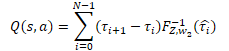
In our particular case, all probability deltas have already been calculated in the cSoftMax buffer with layer results. Now we only have to element-by-element multiply the value of the specified buffer by the result buffer of the quantile function perceptron from the cQuantile2 neural layer. We will summarize the result of the operation in the context of the agent's possible actions.
To perform these operations, we will create a new kernel FQF_Output. In the kernel parameters, we will pass pointers to three data buffers: quantile function results, probability deltas and results buffer. We also indicate the number of quantiles.
We will run the kernel in a one-dimensional task space, which corresponds to the number of possible agent actions.
In the kernel body, we first request a thread identifier and determine the shift in the data buffers to the corresponding quantile distribution vector.
Next, we multiply the probability vector by the quantile distribution vector in a loop. The result of the operation is written to the corresponding result buffer.
Note that the result buffer will be significantly smaller than the original data buffers, since it only contains one discrete value for each possible action. In contrast, the source data contains a whole vector of values for each action. Accordingly, the offset in the result buffer is equal to the identifier of the current thread.
__kernel void FQF_Output(__global float* quantiles,
                         __global float* delta_taus,
                         __global float* output,
                         uint total)
  {
   size_t action = get_global_id(0);
   int shift = action * total;
//---
   float result = 0;
   for(int i = 0; i < total; i++)
      result += quantiles[shift + i] * delta_taus[shift + i];
   output[action] = result;
  }
We have discussed the entire feed forward algorithm FQF and have created the missing kernels. Now we can return to our class and reproduce the whole algorithm using MQL5. As usual, to perform the feed forward pass, we override the CNeuronFQF::feedForward method.
The feed forward method receives in parameters a pointer to the previous neural layer, the result buffer of which (according to our expectations) contains the embedding of the current system state.
We do not create a source data control block in the method body. Instead, we call feed forward methods of inner neural layers cFraction and cSoftMax. Exclusion of the source data control block in this case does not carry any risks, since each of the called methods has its own control block. We just need to check the results of the called methods.
bool CNeuronFQF::feedForward(CNeuronBaseOCL *NeuronOCL)
  {
   if(!cFraction.FeedForward(NeuronOCL))
      return false;
   if(!cSoftMax.FeedForward(GetPointer(cFraction)))
      return false;
Next, we have to create an embedding of probabilistic levels of quantiles. Here we first call the above created data preparation kernel FQF_Cosine. This kernel runs in a two-dimensional task space. In the first dimension, we indicate the number of quantiles. The second dimension is the number of possible agent actions.
Note that we have not created internal variables for the specified hyperparameters. But the size of the result buffer of our CNeuronFQF layer is equal to the number of possible agent actions. And we can define the number of quantiles as the ratio of the cSoftMax layer results buffer to the number of actions.
Pass pointers to buffers to the kernel parameters and add the kernel to the execution queue. Do not forget to control operations at each step.
     {
      uint global_work_offset[2] = {0, 0};
      uint global_work_size[2];
      global_work_size[1] = Output.Total();
      global_work_size[0] = cSoftMax.Neurons() / global_work_size[1];
      OpenCL.SetArgumentBuffer(def_k_FQF_Cosine, def_k_fqf_cosine_softmax, cSoftMax.getOutputIndex());
      OpenCL.SetArgumentBuffer(def_k_FQF_Cosine, def_k_fqf_cosine_outputs, cCosine.getOutputIndex());
      if(!OpenCL.Execute(def_k_FQF_Cosine, 2, global_work_offset, global_work_size))
        {
         printf("Error of execution kernel FQF_Cosine: %d", GetLastError());
         return false;
        }
     }
Next, we call the cCosineEmbeding inner neural layer feed forward method, which completes the quantile embedding process.
   if(!cCosineEmbeding.FeedForward(GetPointer(cCosine)))
      return false;
In the next step of the FQF algorithm we have to combine the embedding of the current system state (initial data) with quantile embedding. As you remember, for this operation we decided to use the Dropout neural layer kernel. In the body of this kernel, we used vector operations for 40element vectors. Therefore, the number of threads will be four times less than the size of the data buffers.
Pass the necessary data in the kernel parameters. Then put the kernel in the execution queue.
     {
      uint global_work_offset[1] = {0};
      uint global_work_size[1] = {(cCosine.Neurons() + 3) / 4};
      OpenCL.SetArgumentBuffer(def_k_Dropout, def_k_dout_input, NeuronOCL.getOutputIndex());
      OpenCL.SetArgumentBuffer(def_k_Dropout, def_k_dout_map, cCosineEmbeding.getOutputIndex());
      OpenCL.SetArgumentBuffer(def_k_Dropout, def_k_dout_out, cQuantile0.getOutputIndex());
      OpenCL.SetArgument(def_k_Dropout, def_k_dout_dimension, (int)cCosine.Neurons());
      if(!OpenCL.Execute(def_k_Dropout, 1, global_work_offset, global_work_size))
        {
         printf("Error of execution kernel Dropout: %d", GetLastError());
         return false;
        }
     }
Now we need to determine the levels of the quantile distribution. To do this, we sequentially call the feed forward methods of the neural layers in our quantile function perceptron.
   if(!cQuantile1.FeedForward(GetPointer(cQuantile0)))
      return false;
//---
   if(!cQuantile2.FeedForward(GetPointer(cQuantile1)))
      return false;
After the feed forward pass method, call the kernel for converting the quantile distribution into a discrete value of the expected reward for each possible agent action FQF_Output. The procedure for putting the kernel in the execution queue is the same:
- define the task space
- pass pointers to buffers and other necessary information to the kernel parameters
- call the kernel execution procedures
Do not forget to control the results at each step.
     {
      uint global_work_offset[1] = {0};
      uint global_work_size[1] = { Neurons() };
      OpenCL.SetArgumentBuffer(def_k_FQF_Output, def_k_fqfout_quantiles, cQuantile2.getOutputIndex());
      OpenCL.SetArgumentBuffer(def_k_FQF_Output, def_k_fqfout_delta_taus, cSoftMax.getOutputIndex());
      OpenCL.SetArgumentBuffer(def_k_FQF_Output, def_k_fqfout_output, getOutputIndex());
      OpenCL.SetArgument(def_k_FQF_Output, def_k_fqfout_total,
                         (uint)(cQuantile2.Neurons() / global_work_size[0]));
      if(!OpenCL.Execute(def_k_FQF_Output, 1, global_work_offset, global_work_size))
        {
         printf("Error of execution kernel FQF_Output: %d", GetLastError());
         return false;
        }
     }
//---
   return true;
  }
This concludes operations with the feed forward kernel. Next, we move on to creating the backpropagation kernels. It is represented by two methods in our class: calcInputGradients and updateInputWeights.
2.2. Feed-Backward
We will first look at the calcInputGradients method in which the gradient is propagated to all internal layers and the previous neural layer.
This method completely repeats the feed forward method, only in the opposite direction. Accordingly, for all the kernels that we created during the direct pass, it is necessary to create kernels with "mirror" operations. Since the entire backpropagation process is a reverse of the feed forward pass, we will build the kernels in the same order.
At the output of the feed forward method, we transformed the quantile distribution into a discrete value for each possible action of the agent. At the input of the backpropagation method, we expect to receive an error gradient for each action. Then we need to distribute the resulting gradient by both the value of the quantile function and the probabilities deltas of the quantile ranges.
We will implement all this in the FQF_OutputGradient kernel. In the kernel parameters, we will pass pointers to five data buffers. Three of them will contain source data and the other two will be used to write kernel operation results.
The delta tensors of probabilities and results of the quantile function are structured with tabular logic in the context of quantiles and possible agent actions. Similarly, we will run the kernel in a two-dimensional task space of quantiles and agent actions.
In the kernel body, we request the thread IDs in both dimensions, the number of treads in the first dimension and determine an offset in the data buffer.
__kernel void FQF_OutputGradient(__global float* quantiles,
                                 __global float* delta_taus,
                                 __global float* output_gr,
                                 __global float* quantiles_gr,
                                 __global float* taus_gr
                                )
  {
   size_t i = get_global_id(0);
   size_t total = get_global_size(0);
   size_t action = get_global_id(1);
   int shift = action * total;
Next, we have to propagate the error gradient. During the feed forward pass, we got the result by multiplying 2 variables. The derivative of the multiplication operation is the second factor. Therefore, to propagate the gradient, we need to multiply the resulting error gradient by the corresponding element of the opposite tensor.
Pay attention that we have to multiply one element of the buffer of the obtained gradients by the corresponding elements of two tensors. That is, we have to access the same element of the global buffer two times. But we remember that accessing the elements of global memory is "expensive". In order to reduce the overall execution time of operations, we will first transfer the value of the global buffer element to the faster private memory variable. Further operations will be performed with this fast variable.
The results of operations will be saved in the corresponding elements of two result buffers.
   float gradient = output_gr[action];
   quantiles_gr[shift + i] = gradient * delta_taus[shift + i];
   taus_gr[shift + i] = gradient * quantiles[shift + i];
  }
The next kernel which we called directly from our feed forward method is Dropout. We performed Hadamard multiplication of two embedding tensors in it: the environment state embedding and the quantile embedding. In the feed forward pass we used the previously created Dropout kernel. Now, to propagate the error gradients in two directions, we would need to call this kernel to times in a row, with different input. However, we are striving for maximum parallelism of operations in order to minimize the model training time. Therefore, let us spend some time and create a new kernel FQF_QuantileGradient.
The algorithm of this kernel completely repeats the algorithm of the previous kernel. There is nothing strange in this. Both kernels perform a similar function. The difference is only in the offset in the buffer of the resulting gradients. In the previous case, the size of the obtained gradients buffer differed from the rest of the buffers since it had only one discrete value for each possible agent action. In this case, all buffers have the same size. And, accordingly, in the buffer of the received gradients, we use an offset as in the rest buffers.
__kernel void FQF_QuantileGradient(__global float* state_embeding,
                                   __global float* taus_embeding,
                                   __global float* quantiles_gr,
                                   __global float* state_gr,
                                   __global float* taus_gr
                                  )
  {
   size_t i = get_global_id(0);
   size_t total = get_global_size(0);
   size_t action = get_global_id(1);
   int shift = action * total;
//---
   float gradient = quantiles_gr[shift + i];
   state_gr[shift + i] = gradient * taus_embeding[shift + i];
   taus_gr[shift + i] = gradient * state_embeding[shift + i];
  }
The last kernel that we have to consider is FQF_CosineGradient, which performs a procedure reverse to preparing data for quantile embedding. The derivative of the data preparation operation is as follows:
![]()
As a result of the operations of this kernel, we expect to get an error gradient at the output of the Softmax layer of the quantile probability prediction model. Pay attention that each quantile used the accumulative value of the Softmax results tensor. This means that each element of the tensor influenced all subsequent quantiles. It would be logical for each element of the tensor to receive its share of the gradient in accordance with its participation in the final result. Therefore, we will collect the error gradient from all elements of the received gradients buffer, which were influenced by the analyzed element of the Softmax results tensor.
Let's consider the implementation of the kernel. In the parameters, we pass pointers to three data buffers:
- Softmax layer results
- obtained error gradients
- results buffer — error gradients at the softmax layer result buffer level
Like most of the kernels discussed in this article, these kernels will run in a two-dimensional task space: one for quantiles and one for possible agent actions.
In the body of the kernel, we request thread IDs in both dimensions and determine the offset in the data buffers. All data buffers are the same size. Consequently, the offset will be the same for all of them.
__kernel void FQF_CosineGradient(__global float* softmax,
                                 __global float* output_gr,
                                 __global float* softmax_gr
                                )
  {
   size_t i = get_global_id(0);
   size_t total = get_global_size(0);
   size_t action = get_global_id(1);
   int shift = action * total;
Each element affects only its own and subsequent quantiles. Therefore, we first calculate the sum of the preceding elements.
   float cumul = 0;
   for(int it = 0; it < i; it++)
      cumul += softmax[shift + it];
Then we calculate the gradient from the corresponding element.
Note that during the feed forward pass, we passed the average value of the quantile to the embedding. Accordingly, we calculate the error gradient based on the average value of the quantile probability.
float result = -M_PI_F * i * sin(M_PI_F * i * (cumul + softmax[shift + i] / 2)) * output_gr[shift + i];
Next, in a loop, we will determine the error gradient from subsequent quantiles. In doing so, we will also adjust the influence of the gradient in accordance with the share of the current element in the total probability of the gradient quantile.
   for(int it = i + 1; it < total; it++)
     {
      cumul += softmax[shift + it - 1];
      float temp = cumul + softmax[shift + it] / 2;
      result += -M_PI_F * it * sin(M_PI_F * it * temp) * output_gr[shift + it] *
                                                         softmax[shift + it] / temp;
     }
   softmax_gr[shift + i] += result;
  }
After all loop iterations, write the result to the corresponding element of the result buffer.
We have prepared all the kernels for organizing the backpropagation pass of our class. So now we can proceed to creating the gradient backpropagation method calcInputGradients.
In the parameters, the method receives a pointer to the object of the previous neural layer to which the error should be propagated. The block of controls is implemented in the method. Here we check pointers to the received object and internal data buffers.
bool CNeuronFQF::calcInputGradients(CNeuronBaseOCL *NeuronOCL)
  {
   if(!NeuronOCL || !Gradient || !Output)
      return false;
Please note that unlike the feed forward method, here we create a control block. This is because the operations of this method begin with the OpenCL program kernel call. When passing it pointers to data buffers, we must be sure that they existence. Otherwise, we can get a critical error in the process of performing operations.
After successfully passing the block of controls, we proceed to the error gradient backpropagation operations. First we call the FQF_OutputGradient kernel, in which we will propagate the error gradient to the quantile function perceptron and the quantile prediction block. The procedure for putting the kernel in the execution queue is similar to that of feed forward: The kernel runs a two-dimensional task space. The first dimension corresponds to quantiles, and the second one to the possible actions of the agent.
     {
      uint global_work_offset[2] = {0, 0};
      uint global_work_size[2] = { cSoftMax.Neurons() / Neurons(), Neurons() };
      OpenCL.SetArgumentBuffer(def_k_FQF_OutputGradient, def_k_fqfoutgr_quantiles,
                                                              cQuantile2.getOutputIndex());
      OpenCL.SetArgumentBuffer(def_k_FQF_OutputGradient, def_k_fqfoutgr_taus,
                                                                 cSoftMax.getOutputIndex());
      OpenCL.SetArgumentBuffer(def_k_FQF_OutputGradient, def_k_fqfoutgr_output_gr,
                                                                 getGradientIndex());
      OpenCL.SetArgumentBuffer(def_k_FQF_OutputGradient, def_k_fqfoutgr_quantiles_gr,
                                                             cQuantile2.getGradientIndex());
      OpenCL.SetArgumentBuffer(def_k_FQF_OutputGradient, def_k_fqfoutgr_taus_gr,
                                                               cSoftMax.getGradientIndex());
      if(!OpenCL.Execute(def_k_FQF_OutputGradient, 2, global_work_offset, global_work_size))
        {
         printf("Error of execution kernel FQF_OutputGradient: %d", GetLastError());
         return false;
        }
     }
Next, we pass the error gradient through the perceptron of the quantile function. To do this, we will sequentially call the backpropagation methods of the inner neural layers of the specified block.
   if(!cQuantile1.calcHiddenGradients(GetPointer(cQuantile2)))
      return false;
   if(!cQuantile0.calcHiddenGradients(GetPointer(cQuantile1)))
      return false;
We have to distribute the error gradient from the quantile function into the current system state embedding (previous neural layer) and quantile probabilities embedding. To perform this functionality, the FQF_QuantileGradient kernel has been created. We call this kernel according to the already similar procedure.
     {
      uint global_work_offset[2] = {0, 0};
      uint global_work_size[2] = { cCosineEmbeding.Neurons(), 1 };
      OpenCL.SetArgumentBuffer(def_k_FQF_QuantileGradient, def_k_fqfqgr_state_enbeding,
                                                                  NeuronOCL.getOutputIndex());
      OpenCL.SetArgumentBuffer(def_k_FQF_QuantileGradient, def_k_fqfqgr_taus_embedding,
                                                            cCosineEmbeding.getOutputIndex());
      OpenCL.SetArgumentBuffer(def_k_FQF_QuantileGradient, def_k_fqfqgr_quantiles_gr,
                                                               cQuantile0.getGradientIndex());
      OpenCL.SetArgumentBuffer(def_k_FQF_QuantileGradient, def_k_fqfqgr_state_gr,
                                                                NeuronOCL.getGradientIndex());
      OpenCL.SetArgumentBuffer(def_k_FQF_QuantileGradient, def_k_fqfqgr_taus_gr,
                                                          cCosineEmbeding.getGradientIndex());
      if(!OpenCL.Execute(def_k_FQF_QuantileGradient, 2, global_work_offset, global_work_size))
        {
         printf("Error of execution kernel FQF_OutputGradient: %d", GetLastError());
         return false;
        }
     }
In the next step we pass the error gradient through quantile embedding. Here we first call the backpropagation method of the inner neural layer cCosine.
   if(!cCosine.calcHiddenGradients(GetPointer(cCosineEmbeding)))
      return false;
Then call FQF_CosineGradient.
     {
      uint global_work_offset[2] = {0, 0};
      uint global_work_size[2] = { cSoftMax.Neurons() / Neurons(), Neurons() };
      OpenCL.SetArgumentBuffer(def_k_FQF_CosineGradient, def_k_fqfcosgr_softmax,
                                                                  cSoftMax.getOutputIndex());
      OpenCL.SetArgumentBuffer(def_k_FQF_CosineGradient, def_k_fqfcosgr_output_gr,
                                                                  cCosine.getGradientIndex());
      OpenCL.SetArgumentBuffer(def_k_FQF_CosineGradient, def_k_fqfcosgr_softmax_gr,
                                                                 cSoftMax.getGradientIndex());
      if(!OpenCL.Execute(def_k_FQF_CosineGradient, 2, global_work_offset, global_work_size))
        {
         printf("Error of execution kernel FQF_CosineGradient: %d", GetLastError());
         return false;
        }
     }
At the end of the method, propagate the error gradient through the inner layer cSoftMax, by calling its backpropagation method.
   if(!cSoftMax.calcInputGradients(GetPointer(cFraction)))
      return false;
//---
   return true;
Pay attention that we do not pass the error gradient from the quantile probabilities prediction block to the previous layer. This is due to the priority of the task related to the determining of the expected reward, rather than the probability distribution.
The second backpropagation method updateInputWeights, which we have to override, is responsible for updating the model parameters. This is quite straightforward. Alternately call the relevant methods of the inner neural layers and check the result of the operations.
bool CNeuronFQF::updateInputWeights(CNeuronBaseOCL *NeuronOCL)
  {
   if(!cFraction.UpdateInputWeights(NeuronOCL))
      return false;
   if(!cCosineEmbeding.UpdateInputWeights(GetPointer(cCosine)))
      return false;
   if(!cQuantile1.UpdateInputWeights(GetPointer(cQuantile0)))
      return false;
   if(!cQuantile2.UpdateInputWeights(GetPointer(cQuantile1)))
      return false;
//---
   return true;
  }
This concludes the work with the main functionality of our new CNeuronFQF class. We have considered the organization of the feed forward and back propagation processes. The methods for saving data to a file and restoring the class have also been overridden in the class. In these methods, we called the corresponding methods of internal objects. You can study them by yourself. You can find the full code of all used classes and their methods in the attachment.
And we're moving on. We have built a class for organizing the model learning algorithm by the method of complete parameterization of the quantile function. But this is only part of the process. This is still the same Q-learning using the data buffer and Target Net. To facilitate the process of using the described method directly in the Q-learning process, we have created the CFQF class derived from our model's base class CNet.
class CFQF : protected CNet
  {
private:
   uint              iCountBackProp;
protected:
   uint              iUpdateTarget;
   //---
   CNet              cTargetNet;
public:
                     CFQF(void);
                     CFQF(CArrayObj *Description)  { Create(Description); }
   bool              Create(CArrayObj *Description);
                    ~CFQF(void);
   bool              feedForward(CArrayFloat *inputVals, int window = 1, bool tem = true)
                     { return        CNet::feedForward(inputVals, window, tem); }
   bool              backProp(CBufferFloat *targetVals, float discount = 0.9f,
                              CArrayFloat *nextState = NULL, int window = 1, bool tem = true);
   void              getResults(CBufferFloat *&resultVals);
   int               getAction(void);
   int               getSample(void);
   float             getRecentAverageError() { return recentAverageError; }
   bool              Save(string file_name, datetime time, bool common = true)
     { return CNet::Save(file_name, getRecentAverageError(), (float)iUpdateTarget, 0, time, common); }
   virtual bool      Save(const int file_handle);
   virtual bool      Load(string file_name, datetime &time, bool common = true);
   virtual bool      Load(const int file_handle);
   //---
   virtual int       Type(void)   const   {  return defFQF;   }
   virtual bool      TrainMode(bool flag) { return CNet::TrainMode(flag); }
   virtual bool      GetLayerOutput(uint layer, CBufferFloat *&result)
     { return        CNet::GetLayerOutput(layer, result); }
   //---
   virtual void      SetUpdateTarget(uint batch)   { iUpdateTarget = batch; }
   virtual bool      UpdateTarget(string file_name);
  };
The class is similar to CQRDQN from the previous article. Its structure is almost identical with the structure of that class. I have removed unused variables and the probability matrix. All this is done in separate neural networks. I have also made the required changes to the class methods. I will not dwell on all the methods of the class now. You can check them yourself in the attachment. I will only mention some of them.
Let us begin with the backpropagation method. The method receives in parameters the target values and the next state of the system. The next state is an optional parameter. It can be used when training a new model, when the use of an untrained model to predict future rewards will cause noise and will complicate the learning process.
In the method body, check the presence of a mandatory parameter in the form of a buffer of target values.
bool CFQF::backProp(CBufferFloat *targetVals, float discount = 0.9f,
                    CArrayFloat *nextState = NULL, int window = 1, bool tem = true)
  {
//---
   if(!targetVals)
      return false;
Then we also check for the presence of an optional parameter and, if necessary, make a prediction of future rewards. Here, we also adjust the target values for the amount of future reward, taking into account the discount factor.
   if(!!nextState)
     {
      vectorf target;
      if(!targetVals.GetData(target) || target.Size() <= 0)
         return false;
      if(!cTargetNet.feedForward(nextState, window, tem))
         return false;
      cTargetNet.getResults(targetVals);
      if(!targetVals)
         return false;
      target = target + discount * targetVals.Maximum();
      if(!targetVals.AssignArray(target))
         return false;
     }
After that check if we need to update Target Net.
   if(iCountBackProp >= iUpdateTarget)
     {
#ifdef FileName
      if(UpdateTarget(FileName + ".nnw"))
#else
      if(UpdateTarget("FQF.upd"))
#endif
         iCountBackProp = 0;
     }
   else
      iCountBackProp++;
At the end of the method, call the parent class's callback method.
   return CNet::backProp(targetVals);
  }
The greedy action selection method has also been changed. Here we simply determine the item with the highest reward from the model's results buffer.
int CFQF::getAction(void)
  {
   CBufferFloat *temp;
   CNet::getResults(temp);
   if(!temp)
      return -1;
//---
   return temp.Maximum(0, temp.Total());
  }
Changes have also been made to the action sampling method getSample. In this method, we first get the result of the last feed forward pass of the model.
int CFQF::getSample(void)
  {
   CBufferFloat* resultVals;
   CNet::getResults(resultVals);
   if(!resultVals)
      return -1;
We copy the received data from the buffer into a vector and apply the Softmax function to them. Then we calculate the cumulative sums of the vector values.
   vectorf temp;
   if(!resultVals.GetData(temp))
     {
      delete resultVals;
      return -1;
     }
   delete resultVals;
//---
   if(!temp.Activation(temp, AF_SOFTMAX))
      return -1;
   temp = temp.CumSum();
The resulting vector is a kind of quantile probability distribution of the agent's actions. Then we sample one value from this distribution and return it to the caller.
   int err_code;
   float random = (float)Math::MathRandomNormal(0.5, 0.5, err_code);
   if(random >= 1)
      return (int)temp.Size() - 1;
   for(int i = 0; i < (int)temp.Size(); i++)
      if(random <= temp[i] && temp[i] > 0)
         return i;
//---
   return -1;
  }
At each step, we check the result of the operations. If an error occurs, return -1 to the calling program.
This concludes the discussion of classes for the implementation of the FQF algorithm. The full code of all classes and their methods is available in the attachment.
3. Testing
To train the model by the method of a fully parameterized quantile function, I have created the FQF-learning.mq5 EA. Its algorithm is very similar to that of QRDQN-learning.mq5 from the previous article. I have only changed the file name and the objects used. So, I will not dwell on its architecture. The full code of the EA is attached below.
The model was trained on the historical data of the EURUSD, for the last 2 years, with the H1 timeframe. All indicators were used with default parameters. As you can see, these are the same parameters we use when testing all models within this series of articles.
During the training process, the model showed a fairly smooth and stable error reduction dynamics. Which is a pretty good marker of model training stability.
The trained model was tested in the strategy tester. A separate EA FQF-learning-test.mq5 was created for testing purposes. It is a copy of QRDQN-learning-test.mq5 from the previous article. So, we will not consider its algorithm now. Only the file name and model class have changed. The full EA code can be found in the attachment.
During testing, the model demonstrated the ability to generate profits. Based on the testing results, the model showed the Profit Factor of 1.78 and the Recovery Factor of 3.7. The share of winning trades exceeds 57%. The largest winning trade is almost 2.5 times higher than the one with the highest loss. The longest winning series had 10 trades, while the longest losing series had 4 trades. In general, the average winning trade is ⅓ higher than the average losing trade.


Conclusion
In this article, we continued studying distributed reinforcement learning algorithms and built classes to implement a Fully Parameterized Quantile Function Learning Method in reinforcement learning. We trained the model using this method and checked the performance of the trained model in the strategy tester. During the learning process, the method demonstrated a steady trend towards error reduction. Testing of the trained model in the strategy tester showed the ability of the model to generate profits.
Once again, I want to remind you that financial market trading is a highly risky investment method. The programs presented in the article are intended only to demonstrate the operation of methods and algorithms. They are not intended for use in live trading. Nevertheless, they can be used as the basis for creating working trading tools. Anyway, before using, you must perform thorough and comprehensive testing of the developed tools. You should understand and accept the risks of using programs in real trading.
References
- Neural networks made easy (Part 3): Convolutional networks
- Neural networks made easy (Part 12): Dropout
- Neural networks made easy (Part 26): Reinforcement learning
- Neural networks made easy (Part 27): Deep Q-Learning (DQN)
- Neural networks made easy (Part 28): Policy gradient algorithm
- Neural networks made easy (Part 32): Distributed Q-Learning
- Neural networks made easy (Part 33): Quantile regression in distributed Q-learning
- A Distributional Perspective on Reinforcement Learning
- Distributional Reinforcement Learning with Quantile Regression
- Implicit Quantile Networks for Distributional Reinforcement Learning
- Fully Parameterized Quantile Function for Distributional Reinforcement Learning
Programs used in the article
| # | Issued to | Type | Description |
|---|---|---|---|
| 1 | FQF-learning.mq5 | EA | EA for optimizing the model |
| 2 | FQF-learning-test.mq5 | EA | An Expert Advisor to test the model in the Strategy Tester |
| 3 | FQF.mqh | Class library | FQF model class |
| 4 | NeuroNet.mqh | Class library | Library for creating neural network models |
| 5 | NeuroNet.cl | Code Base | OpenCL program code library to create neural network models |
| 6 | NetCreator.mq5 | EA | Model building tool |
| 7 | NetCreatotPanel.mqh | Class library | Class library for creating the tool |
Translated from Russian by MetaQuotes Ltd.
Original article: https://www.mql5.com/ru/articles/11804
- Free trading apps
- Over 8,000 signals for copying
- Economic news for exploring financial markets
You agree to website policy and terms of use
Is the nn architecture similar to the one from the previous article except for the last layer?
yes