Neural networks made easy (Part 67): Using past experience to solve new tasks

MetaTrader 5 — Trading systems | 8 April 2024, 14:48

4 453

Dmitriy Gizlyk

Introduction

Reinforcement learning is built on maximizing the reward received from the environment during interaction with it. Obviously, the learning process requires constant interaction with the environment. However, situations are different. When solving some tasks, we can encounter various restrictions on such interaction with the environment. A possible solution for such situations is to use offline reinforcement learning algorithms. They allow you to train models on a limited archive of trajectories collected during preliminary interaction with the environment, while it was available.

Of course, offline reinforcement learning has some drawbacks. In particular, the problem of studying the environment becomes even more acute as we deal with a limited training sample, which is not able to accommodate all the versatility of the environment. This is especially true in complex stochastic environments. In the previous article, we discussed one of the options for solving this tasak (the ExORL metho ).

However, sometimes restrictions on interactions with the environment can be critical. The process of environmental exploration can be accompanied by positive and negative rewards. Negative rewards can be highly undesirable and can be accompanied by financial losses or some other unwanted loss that you cannot accept. But tasks rarely appear out of nowhere. Most often we optimize an existing process. And in our age of information technology, we one can almost always find experience in interacting with the environment being explored in the process of solving tasks similar to the mentioned one. It is possible to use data from real interaction with the environment, which can, to one degree or another, cover the required space of actions and states. Experiments using such experience to solve new tasks when controlling real robots are described in the article "Real World Offline Reinforcement Learning with Realistic Data Source". The authors of the paper propose a new framework for training models: Real-ORL.

1. Real-ORL framework

Offline reinforcement learning (ORL) models a Markov decision environment. This assumes access to a pre-generated dataset in the form of trajectories collected using one or a mixture of behavioral policies. The goal of ORL is to use an offline dataset to train an almost optimal policy π. In general, there is no possibility of learning an optimal policy π* due to insufficient exploration and limited training dataset. In this case, we aim to find the best policy that can be trained based on the available dataset.

Most offline reinforcement learning algorithms include some form of regularization or conservatism. Which may take the following forms, but are not limited to:

Regularization of the policy gradient
Approximate dynamic programming
Learning using an environmental model

The authors of the Real-ORL framework do not offer new model training algorithms. In their work, they explore a range of previously representative ORL algorithms and evaluate their performance on a physical robot in realistic use cases. The authors of the framework note that the learning algorithms analyzed in the article are mostly focused on simulation, using ideal datasets, independent and simultaneous datasets. However, this approach is incorrect in the real stochastic world, in which actions are accompanied by operational delays. This limits the use of trained policies on physical robots. It is unclear whether results from simulated benchmarks or limited equipment evaluations can be generalized to real-world processes. The paper "Real World Offline Reinforcement Learning with Realistic Data Source" aims to fill this gap. It presents empirical studies of several offline reinforcement learning algorithms applied to real-world learning tasks, with an emphasis on generalization beyond the domain of the training set.

In turn, imitation learning is an alternative approach to learning control policies in robotics. Unlike RL, which trains policies by optimizing rewards, imitation learning aims to replicate expert demonstrations. In most cases, it uses supervised learning approaches, which excludes the reward function from the learning process. Also interesting is the combination of reinforcement learning and imitation learning.

In their paper, the authors of the Real-ORL framework use an offline dataset consisting of trajectories from a heuristic manual policy. The trajectories were collected under the supervision of an expert and represent a high-quality dataset. The method authors consider offline imitation learning (in particular behavior cloning) as the basic algorithm in their empirical research.

To maximize objectivity in evaluating learning methods, the article examines four classic manipulative tasks, which represent a set of common manipulative challenges. Each task is modeled as an MDP with a unique reward function. Each of the analyzed learning methods is used to solve all 4 tasks, which puts all algorithms in absolutely equal conditions.

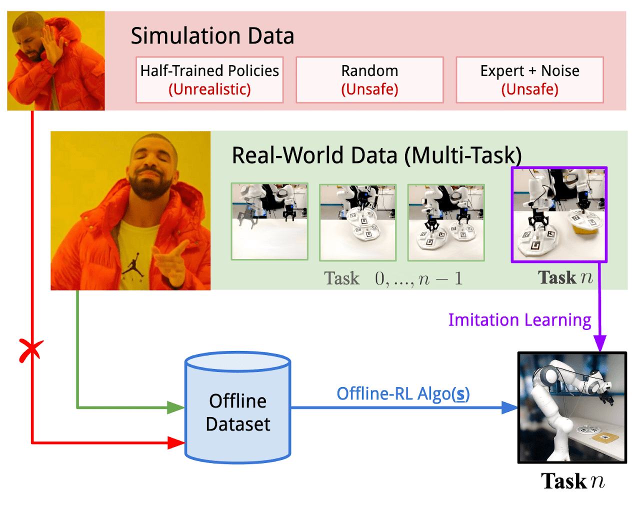
As mentioned above, the training data is collected using a policy developed under the supervision of an expert. Basically, successful trajectories in all four tasks were collected. The authors of the framework believe that collecting suboptimal trajectories or distorting expert trajectories with various noise is not acceptable for robotics, since distorted or random behavior is unsafe and harmful to the technical condition of the equipment. At the same time, the use of data collected from various tasks offers a more realistic environment for applying offline reinforcement learning on real robots for three reasons:

Collecting "random/exploratory" data on a real robot autonomously would require extensive safety restrictions, supervision, and expert guidance.
Using experts to record such random data in large quantities makes less sense than using it to collect meaningful trajectories for a real-world task.
Developing task-specific strategies and stress testing ORL capability against such a strong dataset is more viable than using a compromised dataset.

The authors of the Real-ORL framework, in order to avoid bias in favor of the task (or algorithm), froze the dataset ahead of time.

To train agents' policies in all tasks, the authors of Real-ORL break each task into simpler stages, marked by subgoals. The agent takes small steps toward subgoals until some task-specific criteria are met. Policies trained in this way did not achieve the theoretically maximum possible results due to controller noise and tracking error. However, they complete the task with a high success rate and have performance comparable to human demonstrations.

The authors of Real-ORL conducted experiments that encompassed more than 3000 training trajectories, more than 3500 evaluation trajectories, and more than 270 human labor hours. Through extensive studies, they found that:

For in-domain tasks, reinforcement learning algorithms could be generalized to data-scarce problem domains and to dynamic problems.
The change in ORL performance after using heterogeneous data tends to vary depending on agents, task design, and data characteristics.
Certain heterogeneous, task-independent trajectories can provide overlapping data support and enable better learning, allowing ORL agents to improve their performance.
The best agent for each task is either the ORL algorithm or the parity between ORL and BC. The evaluations presented in the paper indicate that even in an out-of-domain data mode, which is more realistic for the real world, offline reinforcement learning is an effective approach.

Below is the visualization of the Real-ORL framework provided by the authors.

2. Implementation using MQL5

The paper "Real World Offline Reinforcement Learning with Realistic Data Source" empirically confirms the effectiveness of offline reinforcement learning methods for solving real-world tasks. But what caught my attention was the use of data on solving similar tasks to build the Agent policy. The only criterion for data here is the environment. That is, the dataset must be collected as a result of interaction with the environment we are analyzing.

How can we benefit from this? At least, we receive extensive information about the exploration of the environment, in our case financial markets. We have talked many times about one of the main tasks of reinforcement learning which is environmental exploration. At the same time, we always had a huge amount of information that we did not use. I'm talking about signals. In the screenshot below, I intentionally removed the authors and the names of the signals. In our experiment, the only criterion for signals is the presence of transactions during the historical period of the training period for the selected financial instrument.

Signals

We train models on the time period for the first 7 months of 2023 of the EURUSD instrument. These criteria will be used to select signals. These can be both paid and free signals. Please note that in paid signals, part of the history is hidden. However, usually the latest deals are hidden. But we are interested in open history.

On the "Account" tab, we check for the operations in the period of interest.

On the "Statistics" tab, we check for the operations for the financial instrument. But we are not looking for signals that work only for the instrument of interest. We will exclude unnecessary deals later.

I agree that this is a rather approximate and indirect analysis. It does not guarantee the presence of deals for the analyzed financial instrument in the desired historical period. But the likelihood that there are deals is quite high. This analysis is quite simple and easy to perform.

When we find a suitable signal, we go to the signal's "Deal history" tab and download a csv file with the operation history.

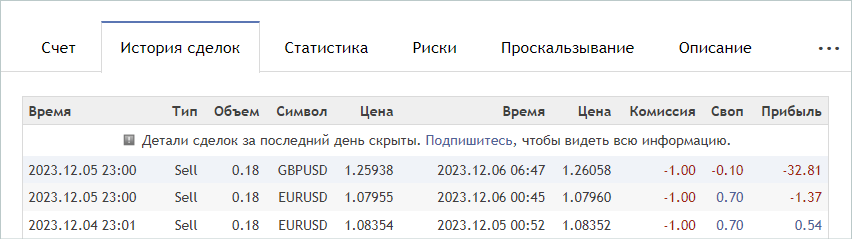
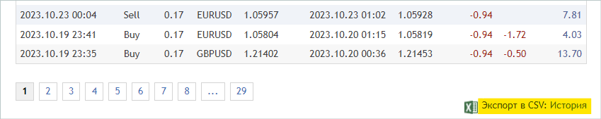
Please note that downloaded files must be saved in the MetaTrader 5 common folder "...\AppData\Roaming\MetaQuotes\Terminal\Common\Files\". For ease of use, I created a subdirectory "Signals" and renamed the files of all signals to "SignalX.csv" where X is a serial number of the saved signal history.

It should be noted here that the Real-ORL framework under consideration involves the use of selected trajectories as the experience of interaction with the environment. By no means does it promise complete cloning of trajectories. Therefore, when selecting trajectories, we do not check the correlation (or any other statistical analysis) of deals with the indicators we use. For the same reason, you should not expect a trained model to completely repeat the actions of the most profitable or any other signal used.

Using this method, I selected 20 signals. However, we cannot use the resulting csv files as they are to train our models. We need to map deals to historical price movement data and indicator readings at the time of deals and collect trajectories for each of the signals used. We will perform this functionality in the Expert Advisor "...\RealORL\ResearchRealORL.mq5", but first we will do a little preparatory work.

To record each trade transaction from the signal's trade history, we will create a CDeal class. This class is intended for internal use only. To eliminate unnecessary operations, we will omit the wrappers for accessing class variables. All variables will be declared publicly.

class CDeal       :  public CObject
  {
public:
   datetime             OpenTime;
   datetime             CloseTime;
   ENUM_POSITION_TYPE   Type;
   double               Volume;
   double               OpenPrice;
   double               StopLos;
   double               TakeProfit;
   double               point;
   //---
                        CDeal(void);
                       ~CDeal(void) {};
   //---
   vector<float>        Action(datetime current, double ask, double bid, int period_seconds);
  };

Class variables are comparable to DEAL fields in MetaTrader 5. We have only omitted the variable for the symbol name, since we are supposed to work with one financial symbol. However, if you are building a multi-currency model, you should add the symbol name.

Also note that in the deal, we specify the stop loss and the take profit in the form of a price, while the model generates the Agent's action in relative units. To be able to convert data, we will store the size of one symbol point in the point variable.

In the class constructor, we will fill the variables with initial values. The class destructor remains empty.

void CDeal::CDeal(void) :  OpenTime(0),
                           CloseTime(0),
                           Type(POSITION_TYPE_BUY),
                           Volume(0),
                           OpenPrice(0),
                           StopLos(0),
                           TakeProfit(0),
                           point(1e-5)
  {
  }

To convert a deal into a vector of Agent actions, we will create the Action method. In its parameters, we will pass the current bar opening date and time, bid and ask prices, as well as the interval of the analyzed timeframe in seconds. We always perform market analysis and all trading operations at the opening of each bar.

Pay attention that the time of trading operations in the history of the signals we collected may differ from the opening time of the bar in the timeframe we use. If we can close a position using a stop loss or take profit inside the bar, then we can open a position only at the opening of the bar. Therefore, here we make an assumption and a small adjustment to the position opening price and time: we open a position at the opening of the bar if in the signal history it opens before it closes.

Following this logic, in the method code, if the current time is less than the position opening time taking into account the adjustment or greater than the position closing time, then the method will return a zero vector of Agent actions.

vector<float> CDeal::Action(datetime current, double ask, double bid, int period_seconds)
  {
   vector<float> result = vector<float>::Zeros(NActions);
   if((OpenTime - period_seconds) > current || CloseTime <= current)
      return result;

Please note that we first create a null vector of results, and only then implement time control and return the result. This approach allows us to further operate with the generated zero vector of results. Therefore, if it is necessary to fill the action vector, we fill only non-zero elements.

The action vector is populated in the body of the switch selection statement depending on the type of position. In the case of a long position, we record the operation volume in the element indexed with 0. Then we check the take profit and stop loss to see if they are different from 0 and, if necessary, convert the price to a relative value. Write the resulting values into elements with indexes 1 and 2, respectively.

   switch(Type)
     {
      case POSITION_TYPE_BUY:
         result[0] = float(Volume);
         if(TakeProfit > 0)
            result[1] = float((TakeProfit - ask) / (MaxTP * point));
         if(StopLos > 0)
            result[2] = float((ask - StopLos) / (MaxSL * point));
         break;

Similar operations are performed for a short position, but with the indexes of the vector elements shifted by 3.

      case POSITION_TYPE_SELL:
         result[3] = float(Volume);
         if(TakeProfit > 0)
            result[4] = float((bid - TakeProfit) / (MaxTP * point));
         if(StopLos > 0)
            result[5] = float((StopLos - bid) / (MaxSL * point));
         break;
     }

The generated vector is returned to the caller.

//---
   return result;
  }

We will combine all deals of one signal in the CDeals class. This class will contain a dynamic array of objects, to which we will add instances of the above created CDeal class and 2 methods:

LoadDeals to load deals from a csv history file;
Action to generate a vector of the Agent's actions.

class CDeals
  {
protected:
   CArrayObj         Deals;
public:
                     CDeals(void) { Deals.Clear(); }
                    ~CDeals(void) { Deals.Clear(); }
   //---
   bool              LoadDeals(string file_name, string symbol, double point);
   vector<float>     Action(datetime current, double ask, double bid, int period_seconds);
  };

In the class constructor and destructor, we clear the dynamic array of deals.

I propose to start considering the methods of the class by loading the deal history from the csv file LoadDeals. In the method parameters, we pass the file name, the name of the analyzed instrument and the point size. I deliberately included the symbol name in the parameters, since there are often differences in the names of financial instruments with different brokers. Consequently, even when the Expert Advisor is running on the chart of the analyzed instrument, its name may differ from the signal unified in the history file.

bool CDeals::LoadDeals(string file_name, string symbol, double point)
  {
   if(file_name == NULL || !FileIsExist(file_name, FILE_COMMON))
     {
      PrintFormat("File %s not exist", file_name);
      return false;
     }

In the body of the method, we first check the file name and its presence in the common terminal folder. If the required file is not found, inform the user and complete the method with the false result.

bool CDeals::LoadDeals(string file_name, string symbol, double point)
  {
   if(file_name == NULL || !FileIsExist(file_name, FILE_COMMON))
     {
      PrintFormat("File %s not exist", file_name);
      return false;
     }

The next step is to check the name of the specified financial symbol. If the name is not found, write the symbol name of the chart on which the EA is running.

   if(symbol == NULL)
     {
      symbol = _Symbol;
      point = _Point;
     }

After successfully passing the control block, open the file specified in the method parameters and immediately check the result of the operation using the received handle value. If for some reason the file cannot be opened, inform the user about the error that has occurred and terminate the method with a negative result.

   ResetLastError();
   int handle = FileOpen(file_name, FILE_READ | FILE_ANSI | FILE_CSV | FILE_COMMON, short(';'), CP_ACP);
   if(handle == INVALID_HANDLE)
     {
      PrintFormat("Error of open file %s: %d", file_name, GetLastError());
      return false;
     }

At this point, the preparatory work stage is completed, and we move on to organizing the data reading cycle. Before each iteration of the loop, we check whether the end of the file has been reached.

   FileSeek(handle, 0, SEEK_SET);
   while(!FileIsEnding(handle))
     {
      string s = FileReadString(handle);
      datetime open_time = StringToTime(s);
      string type = FileReadString(handle);
      double volume = StringToDouble(FileReadString(handle));
      string deal_symbol = FileReadString(handle);
      double open_price = StringToDouble(FileReadString(handle));
      volume = MathMin(volume, StringToDouble(FileReadString(handle)));
      datetime close_time = StringToTime(FileReadString(handle));
      double close_price = StringToDouble(FileReadString(handle));
      s = FileReadString(handle);
      s = FileReadString(handle);
      s = FileReadString(handle);

In the body of the loop, we first read all the information for one transaction and write it to local variables. According to the file structure, the last 3 elements contain the commission, swap and profit for the deal. We do not use this data in our trajectory since the opening time and price may differ from those indicated in the history. Thus, the profit values may also differ. In addition, commissions and swaps depend on the broker's settings.

Next, we check the correspondence of the financial instrument of the trading operation and the one we are analyzing, which was passed in the parameters. If the symbols do not match, move on to the next iteration of the loop.

      if(StringFind(deal_symbol, symbol, 0) < 0)
         continue;

If a deal was performed on the desired financial instrument, we create an instance of the deal description object.

      ResetLastError();
      CDeal *deal = new CDeal();
      if(!deal)
        {
         PrintFormat("Error of create new deal object: %d", GetLastError());
         return false;
        }

Then we fill it. However, please mind the following. We can easily save:

position type
opening and closing times
open price
trade volume
size of one point

But the stop loss and take profit prices are not indicated in the trading history. Instead, only the price of the actual closing of the position is indicated. We will use pretty simple logic here:

We introduce the assumption that the position was closed by stop loss or take profit.
In this case, if the position was closed with a profit, then it was closed at take profit. Otherwise, it was closed at stop loss. In the appropriate field, indicate the closing price.
The opposite field remains empty.

      deal.OpenTime = open_time;
      deal.CloseTime = close_time;
      deal.OpenPrice = open_price;
      deal.Volume = volume;
      deal.point = point;
      if(type == "Sell")
        {
         deal.Type = POSITION_TYPE_SELL;
         if(close_price < open_price)
           {
            deal.TakeProfit = close_price;
            deal.StopLos = 0;
           }
         else
           {
            deal.TakeProfit = 0;
            deal.StopLos = close_price;
           }
        }
      else
        {
         deal.Type = POSITION_TYPE_BUY;
         if(close_price > open_price)
           {
            deal.TakeProfit = close_price;
            deal.StopLos = 0;
           }
         else
           {
            deal.TakeProfit = 0;
            deal.StopLos = close_price;
           }
        }

I fully understand the risks of trading without stop losses, but at the same time I expect this to be minimized during downstream training of the model.

We add the created deal description to a dynamic array and move on to the next iteration of the loop.

      ResetLastError();
      if(!Deals.Add(deal))
        {
         PrintFormat("Error of add new deal: %d", GetLastError());
         return false;
        }
     }

After reaching the end of the file, we close it and exit the method with the result true.

   FileClose(handle);
//---
   return true;
  }

The algorithm for generating the Agent's action vector is quite simple. We go through the entire array of deals and call the appropriate methods for each deal.

vector<float> CDeals::Action(datetime current, double ask, double bid, int period_seconds)
  {
   vector<float> result = vector<float>::Zeros(NActions);
   for(int i = 0; i < Deals.Total(); i++)
     {
      CDeal *deal = Deals.At(i);
      if(!deal)
         continue;
      vector<float> action = deal.Action(current, ask, bid, period_seconds);

However, there are some nuances. We assume that in the history of a signal several positions can be opened simultaneously, including those in different directions. Therefore, we need to add up the vectors obtained from all deals from the archive. But we can only add volumes. Simply adding stop loss and take profit levels will be incorrect. Remember that in the Agent's action vector, stop loss and take profit are specified as shift in relative units from the current price. Thus, when adding the vectors for the stop loss and take profit levels, we take the maximum deviation. Volumes that were not closed on time will be closed by the EA at the opening of a new candlestick, since in this case we expect a decrease in the total volume of the total position.

      result[0] += action[0];
      result[3] += action[3];
      result[1] = MathMax(result[1], action[1]);
      result[2] = MathMax(result[2], action[2]);
      result[4] = MathMax(result[4], action[4]);
      result[5] = MathMax(result[5], action[5]);
     }
//---
   return result;
  }

We pass the final vector of Agent actions to the calling program and terminate the method.

With this we complete the preparatory work and move on to working on the Expert Advisor "...\RealORL\ResearchRealORL.mq5". This EA was created on the basis of the previously discussed EAs "...\...\Research.mq5" and thus it inherited their construction template. It also inherited all external parameters.

//+------------------------------------------------------------------+
//| Input parameters                                                 |
//+------------------------------------------------------------------+
input ENUM_TIMEFRAMES      TimeFrame   =  PERIOD_H1;
input double               MinProfit   =  -10000;
//---
input group                "---- RSI ----"
input int                  RSIPeriod   =  14;            //Period
input ENUM_APPLIED_PRICE   RSIPrice    =  PRICE_CLOSE;   //Applied price
//---
input group                "---- CCI ----"
input int                  CCIPeriod   =  14;            //Period
input ENUM_APPLIED_PRICE   CCIPrice    =  PRICE_TYPICAL; //Applied price
//---
input group                "---- ATR ----"
input int                  ATRPeriod   =  14;            //Period
//---
input group                "---- MACD ----"
input int                  FastPeriod  =  12;            //Fast
input int                  SlowPeriod  =  26;            //Slow
input int                  SignalPeriod =  9;            //Signal
input ENUM_APPLIED_PRICE   MACDPrice   =  PRICE_CLOSE;   //Applied price
//---
input int                  Agent      = 1;

At the same time, this EA does not use any model, since the decision on trading operations has already been made for us, and we use the history of signal deals. Therefore, we remove all model objects and add one CDeals signal deal array object.

SState               sState;
STrajectory          Base;
STrajectory          Buffer[];
STrajectory          Frame[1];
CDeals               Deals;
//---
float                dError;
datetime             dtStudied;
//---
CSymbolInfo          Symb;
CTrade               Trade;
//---
MqlRates             Rates[];
CiRSI                RSI;
CiCCI                CCI;
CiATR                ATR;
CiMACD               MACD;
//---
double               PrevBalance = 0;
double               PrevEquity = 0;

Similarly, in the EA initialization method, instead of loading a pre-trained model, we load the history of trading operations.

//+------------------------------------------------------------------+
//| Expert initialization function                                   |
//+------------------------------------------------------------------+
int OnInit()
  {
//---
   if(!Symb.Name(_Symbol))
      return INIT_FAILED;
   Symb.Refresh();
//---
   if(!RSI.Create(Symb.Name(), TimeFrame, RSIPeriod, RSIPrice))
      return INIT_FAILED;
//---
   if(!CCI.Create(Symb.Name(), TimeFrame, CCIPeriod, CCIPrice))
      return INIT_FAILED;
//---
   if(!ATR.Create(Symb.Name(), TimeFrame, ATRPeriod))
      return INIT_FAILED;
//---
   if(!MACD.Create(Symb.Name(), TimeFrame, FastPeriod, SlowPeriod, SignalPeriod, MACDPrice))
      return INIT_FAILED;
   if(!RSI.BufferResize(HistoryBars) || !CCI.BufferResize(HistoryBars) ||
      !ATR.BufferResize(HistoryBars) || !MACD.BufferResize(HistoryBars))
     {
      PrintFormat("%s -> %d", __FUNCTION__, __LINE__);
      return INIT_FAILED;
     }
//---
   if(!Trade.SetTypeFillingBySymbol(Symb.Name()))
      return INIT_FAILED;
//--- load history
   if(!Deals.LoadDeals(SignalFile(Agent), "EURUSD", SymbolInfoDouble(_Symbol, SYMBOL_POINT)))
      return INIT_FAILED;
//---
   PrevBalance = AccountInfoDouble(ACCOUNT_BALANCE);
   PrevEquity = AccountInfoDouble(ACCOUNT_EQUITY);
//---
   return(INIT_SUCCEEDED);
  }

Note that when downloading signal deals data, instead of the file name, we indicate SignalFile(Agent). Here we use macro substitution. This is why we previously created unified signal file names "SignalX.csv". Macro substitution returns the unified name of the signal history file indicating the value of the external Agent parameter as an identifier.

#define        SignalFile(agent)       StringFormat("Signals\\Signal%d.csv",agent)

This allows us to subsequently run "...\RealORL\ResearchRealORL.mq5" in the optimization mode in the MetaTrader 5 strategy tester. Optimization by the Agent parameter will allow each pass to work with its own signal history file. This way we will be able to process several signal files in parallel and collect trajectories of interaction with the environment from them.

Interaction with the environment is implemented in the OnTick method. Here, as usual, we first check the occurrence of the new bar opening event.

void OnTick()
  {
//---
   if(!IsNewBar())
      return;

If necessary, we download historical price movement data. We also update the buffers of objects for working with indicators.

   int bars = CopyRates(Symb.Name(), TimeFrame, iTime(Symb.Name(), TimeFrame, 1), HistoryBars, Rates);
   if(!ArraySetAsSeries(Rates, true))
      return;
//---
   RSI.Refresh();
   CCI.Refresh();
   ATR.Refresh();
   MACD.Refresh();
   Symb.Refresh();
   Symb.RefreshRates();

The absence of models for decision making means there is no need to fill data buffers. However, to save information in the trajectory of interaction with the environment, we need to fill the state structure with the necessary data. First, we will collect data on price movement and indicator performance.

   float atr = 0;
   for(int b = 0; b < (int)HistoryBars; b++)
     {
      float open = (float)Rates[b].open;
      float rsi = (float)RSI.Main(b);
      float cci = (float)CCI.Main(b);
      atr = (float)ATR.Main(b);
      float macd = (float)MACD.Main(b);
      float sign = (float)MACD.Signal(b);
      if(rsi == EMPTY_VALUE || cci == EMPTY_VALUE || atr == EMPTY_VALUE || macd == EMPTY_VALUE || sign == EMPTY_VALUE)
         continue;
      //---
      int shift = b * BarDescr;
      sState.state[shift] = (float)(Rates[b].close - open);
      sState.state[shift + 1] = (float)(Rates[b].high - open);
      sState.state[shift + 2] = (float)(Rates[b].low - open);
      sState.state[shift + 3] = (float)(Rates[b].tick_volume / 1000.0f);
      sState.state[shift + 4] = rsi;
      sState.state[shift + 5] = cci;
      sState.state[shift + 6] = atr;
      sState.state[shift + 7] = macd;
      sState.state[shift + 8] = sign;
     }

Then we will enter information about the account status and open positions. We will also indicate the opening time of the current bar. Note that at this stage we only save one time value without creating harmonics of the timestamp. This allows us to reduce the amount of data saved without losing information.

   sState.account[0] = (float)AccountInfoDouble(ACCOUNT_BALANCE);
   sState.account[1] = (float)AccountInfoDouble(ACCOUNT_EQUITY);
//---
   double buy_value = 0, sell_value = 0, buy_profit = 0, sell_profit = 0;
   double position_discount = 0;
   double multiplyer = 1.0 / (60.0 * 60.0 * 10.0);
   int total = PositionsTotal();
   datetime current = TimeCurrent();
   for(int i = 0; i < total; i++)
     {
      if(PositionGetSymbol(i) != Symb.Name())
         continue;
      double profit = PositionGetDouble(POSITION_PROFIT);
      switch((int)PositionGetInteger(POSITION_TYPE))
        {
         case POSITION_TYPE_BUY:
            buy_value += PositionGetDouble(POSITION_VOLUME);
            buy_profit += profit;
            break;
         case POSITION_TYPE_SELL:
            sell_value += PositionGetDouble(POSITION_VOLUME);
            sell_profit += profit;
            break;
        }
      position_discount += profit - (current - PositionGetInteger(POSITION_TIME)) * multiplyer * MathAbs(profit);
     }
   sState.account[2] = (float)buy_value;
   sState.account[3] = (float)sell_value;
   sState.account[4] = (float)buy_profit;
   sState.account[5] = (float)sell_profit;
   sState.account[6] = (float)position_discount;
   sState.account[7] = (float)Rates[0].time;

In the reward vector, we immediately fill the elements of the impact of changes in balance and equity.

   sState.rewards[0] = float((sState.account[0] - PrevBalance) / PrevBalance);
   sState.rewards[1] = float(1.0 - sState.account[1] / PrevBalance);

And save the balance and equity values that we will need on the next bar to calculate the reward.

   PrevBalance = sState.account[0];
   PrevEquity = sState.account[1];

Instead of a feed-forward pass of the Agent, we request a vector of actions from the history of signal deals.

   vector<float> temp = Deals.Action(TimeCurrent(), 
                                     SymbolInfoDouble(_Symbol, SYMBOL_ASK), 
                                     SymbolInfoDouble(_Symbol, SYMBOL_BID), 
                                     PeriodSeconds(TimeFrame)
                                    );

Processing and decoding of the action vector are implemented according to the algorithm prepared earlier. First, we exclude multidirectional volumes.

   double min_lot = Symb.LotsMin();
   double step_lot = Symb.LotsStep();
   double stops = MathMax(Symb.StopsLevel(), 1) * Symb.Point();
   if(temp[0] >= temp[3])
     {
      temp[0] -= temp[3];
      temp[3] = 0;
     }
   else
     {
      temp[3] -= temp[0];
      temp[0] = 0;
     }

We then adjust the long position. But previously we did not allow the possibility of opening a position without specifying a stop loss or take profit. This is a necessary measure now. Therefore, we make adjustments in terms of checking the closure of previously open positions and indicating stop loss / take profit prices.

//--- buy control
   if(temp[0] < min_lot || (temp[1] > 0 && (temp[1] * MaxTP * Symb.Point()) <= stops) || 
                           (temp[2] > 0 && (temp[2] * MaxSL * Symb.Point()) <= stops))
     {
      if(buy_value > 0)
         CloseByDirection(POSITION_TYPE_BUY);
     }
   else
     {
      double buy_lot = min_lot + MathRound((double)(temp[0] - min_lot) / step_lot) * step_lot;
      double buy_tp = (temp[1] > 0 ? NormalizeDouble(Symb.Ask() + temp[1] * MaxTP * Symb.Point(), Symb.Digits()) : 0);
      double buy_sl = (temp[2] > 0 ? NormalizeDouble(Symb.Ask() - temp[2] * MaxSL * Symb.Point(), Symb.Digits()) : 0);
      if(buy_value > 0)
         TrailPosition(POSITION_TYPE_BUY, buy_sl, buy_tp);
      if(buy_value != buy_lot)
        {
         if(buy_value > buy_lot)
            ClosePartial(POSITION_TYPE_BUY, buy_value - buy_lot);
         else
            Trade.Buy(buy_lot - buy_value, Symb.Name(), Symb.Ask(), buy_sl, buy_tp);
        }
     }

We make similar adjustments in the short position adjustment block.

//--- sell control
   if(temp[3] < min_lot || (temp[4] > 0 && (temp[4] * MaxTP * Symb.Point()) <= stops) || 
                           (temp[5] > 0 && (temp[5] * MaxSL * Symb.Point()) <= stops))
     {
      if(sell_value > 0)
         CloseByDirection(POSITION_TYPE_SELL);
     }
   else
     {
      double sell_lot = min_lot + MathRound((double)(temp[3] - min_lot) / step_lot) * step_lot;;
      double sell_tp = (temp[4] > 0 ? NormalizeDouble(Symb.Bid() - temp[4] * MaxTP * Symb.Point(), Symb.Digits()) : 0);
      double sell_sl = (temp[5] > 0 ? NormalizeDouble(Symb.Bid() + temp[5] * MaxSL * Symb.Point(), Symb.Digits()) : 0);
      if(sell_value > 0)
         TrailPosition(POSITION_TYPE_SELL, sell_sl, sell_tp);
      if(sell_value != sell_lot)
        {
         if(sell_value > sell_lot)
            ClosePartial(POSITION_TYPE_SELL, sell_value - sell_lot);
         else
            Trade.Sell(sell_lot - sell_value, Symb.Name(), Symb.Bid(), sell_sl, sell_tp);
        }
     }

At the end of the method, we add data to the reward vector, copy the action vector, and pass the structure to be added to the trajectory.

   if((buy_value + sell_value) == 0)
      sState.rewards[2] -= (float)(atr / PrevBalance);
   else
      sState.rewards[2] = 0;
   for(ulong i = 0; i < NActions; i++)
      sState.action[i] = temp[i];
   sState.rewards[3] = 0;
   sState.rewards[4] = 0;
   if(!Base.Add(sState))
      ExpertRemove();
  }

This concludes our review of the methods of the EA "...\RealORL\ResearchRealORL.mq5", since the remaining methods are used without changes. The full code of the EA and all programs used in the article is available in the attachment.

The authors of the Real-ORL method do not propose a new method for learning the Actor policy. For our experiment, we did not make changes either to the policy learning algorithm or to the model architecture. We take this step consciously to make the conditions comparable to training the model from the previous article. Ultimately this will allow us to evaluate the impact of the Real-ORL framework itself on the result of policy learning.

3. Testing

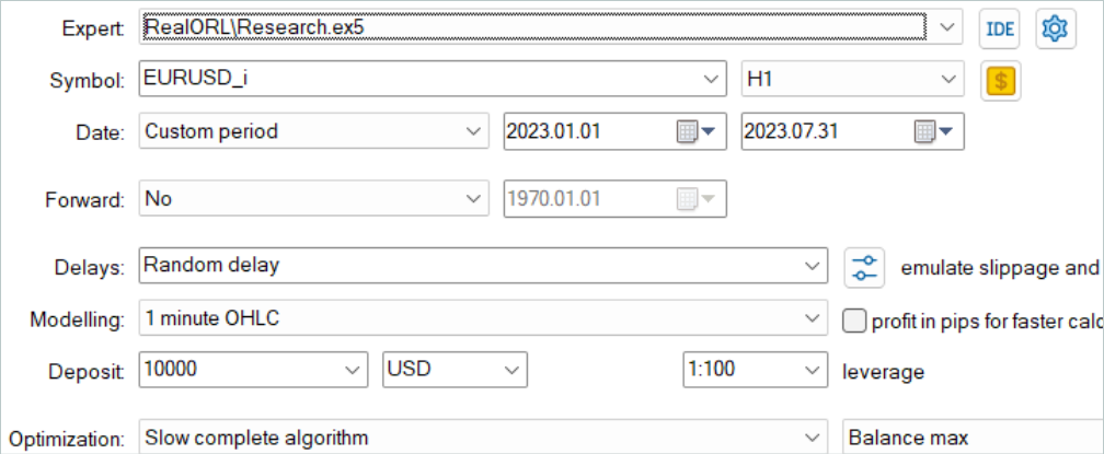
Above, we collected information about trading operations of various signals and prepared an Expert Advisor to transform the collected information into trajectories of interaction with the environment. Now we move on to testing the work done and assessing the impact of the selected trajectories on the model training results. In this work, we will train completely new models initialized with random parameters. In the previous article, we optimized previously trained models.

First, we run the EA for converting the history of signals into the trajectory "...\RealORL\ResearchRealORL.mq5". We will run the EA in full optimization mode.

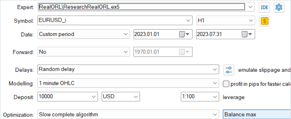
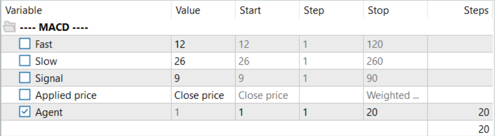
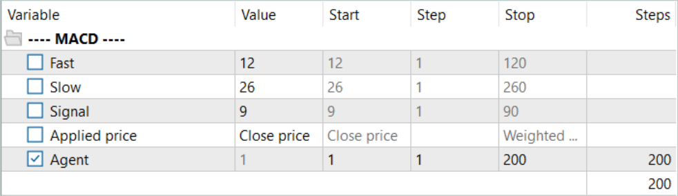
We will optimize it for only one parameter Agent. In the parameter range we will indicate the first and last ID of the signal files in increments of "1".

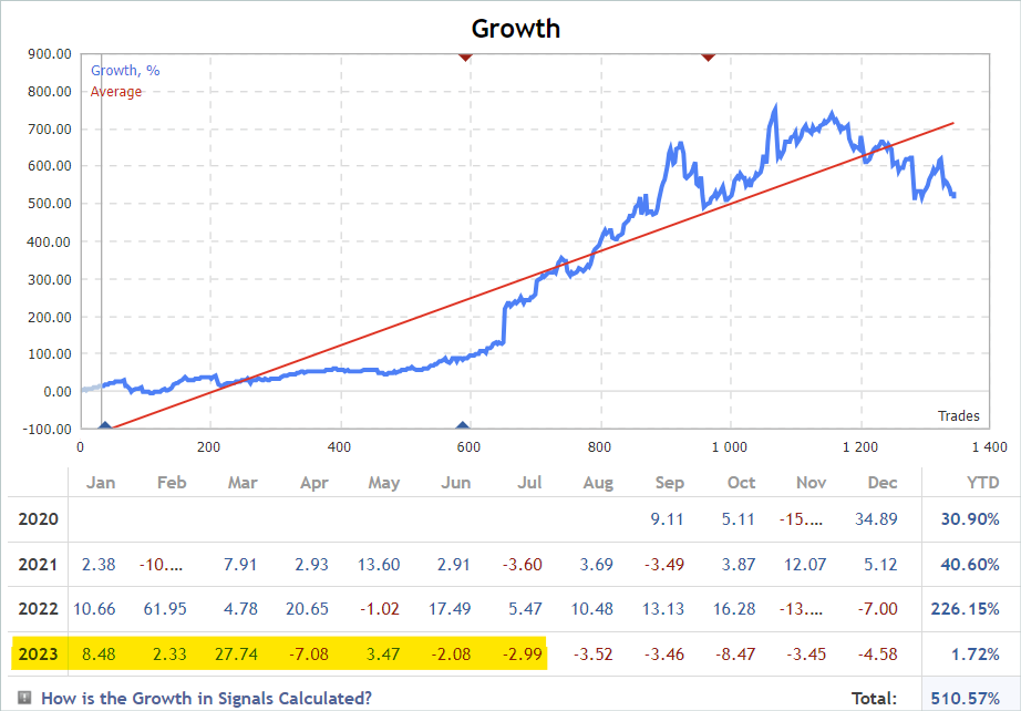
The result was some pretty interesting trajectories.

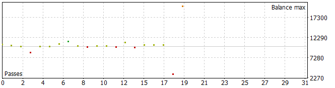
Five of the passes during the analyzed period closed with a loss, and one doubled its balance.

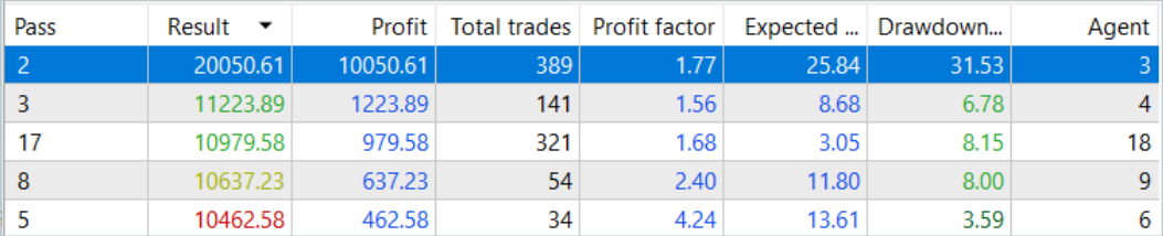
A single pass of the most profitable trajectory showed a fairly deep drawdown on 02/07/2023 and 07/25/2023. I will not discuss the strategy used by the author of the signal, since I am not familiar with it. In addition, it is quite possible that the drawdown is caused by an early opening of a position, provoked by a shift in the position opening point to the beginning of the bar of the analyzed timeframe. And, of course, the use of stop losses, which we deliberately reset to zero, will lead to locking in losses in such situations.

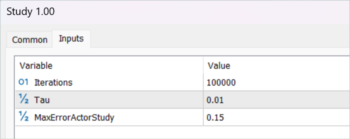
After saving the trajectories, we move on to training the model. To do this, we run the EA "...\RealORL\Study.mq5".

Primary training was performed only on trajectory data collected from the results of signal operation. I must admit that a miracle did not happen. The model results after initial training were far from desired. The trained policy generated a loss both for the training period in the first 7 months of 2023 and for the test historical interval for August 2023. But I would not talk about the ineffectiveness of the proposed Real-ORL framework. The selected 20 trajectories are far from the 3000 trajectories used by the authors of the framework. These 20 trajectories do not cover even a small part of the variety of possible actions of the agent.

Before continuing training, more data was added to the buffer of training trajectories using the EA "...\RealORL\Research.mq5". This EA advisor executes passes with decision-making based on the Agent's pre-trained policy. The exploration of the environment is performed thanks to the stochasticity of the Agent's latent state and policy. Two stochasticities create a fairly large variety of Agent actions, which makes it possible to explore the environment. As the Agent's policy learns, both stochasticities decrease due to a decrease in the variance of each parameter. This makes the Agent's actions more predictable and conscious.

We add 200 new trajectories to the buffer and repeat the model training process.

This time, the Agent policy training process was quite lengthy. I had to update the experience replay buffer many times using the "...\RealORL\Research.mq5" EA before I got a profitable policy. Please note that in the process of updating the experience replay buffer after it is completely filled, we replace the highest-loss (lowest-profit) trajectories with more profitable ones. Consequently, we only replaced trajectories collected using the "...\RealORL\Research.mq5" EA. The trajectories from the signals, due to their general profitability, constantly remained in the experience replay buffer.

As mentioned earlier, as a result of long training, I managed to obtain a policy that was capable of generating profit on the training set. Moreover, the resulting policy was able to generalize the experience gained to new data. This is evidenced by the profit on historical data beyond the training period.

Test results

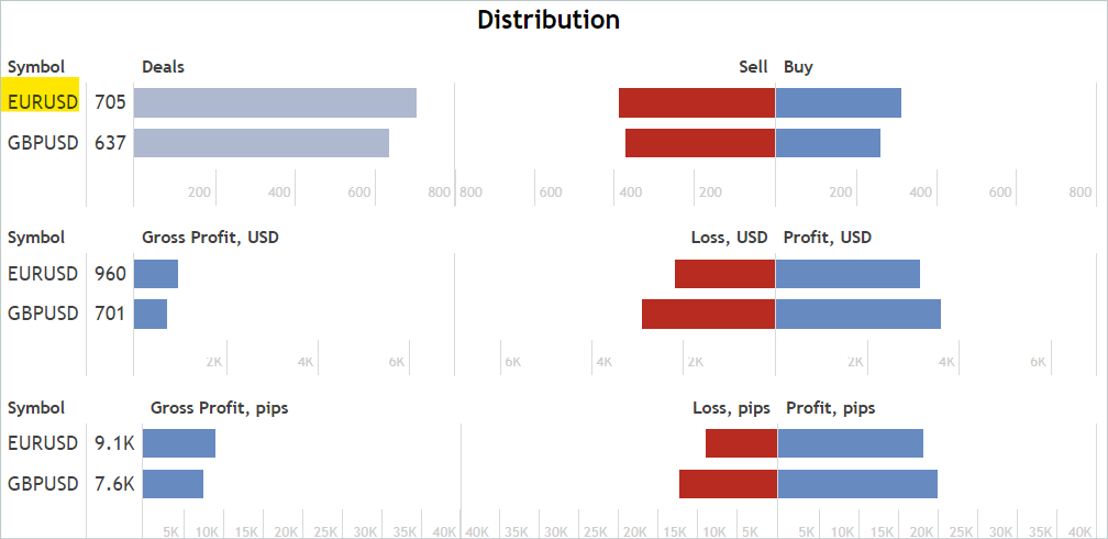
Based on the historical data of the test sample, the Agent made 131 transactions, 48.85% of which were closed with a profit. The maximum profitable trade is almost 10% lower than the maximum loss (379.89 versus 398.49, respectively). At the same time, the average profitable trade is 40% higher than the average loss. As a result, the profit factor for the testing period was 1.34, and the recovery factor was 0.94.

It should also be noted that there is almost parity between long (70) and short (61) transactions. This demonstrates the Agent's ability to highlight local trends, and not just follow the global trend.

Conclusion

In this article, we discussed the Real-ORL framework, which came to us from robotics. The authors of the framework conduct quite extensive empirical research in their work using a real robot, which allows them to draw the following conclusions:

For in-domain tasks, reinforcement learning algorithms could be generalized to data-scarce problem domains and to dynamic problems.
The change in ORL performance after using heterogeneous data tends to vary depending on agents, task design, and data characteristics.
Certain heterogeneous, task-independent trajectories can provide overlapping data support and enable better learning, allowing ORL agents to improve their performance.
The best agent for each task is either the ORL algorithm or the parity between ORL and BC. The evaluations presented in the paper indicate that even in an out-of-domain data mode, which is more realistic for the real world, offline reinforcement learning is an effective approach.

In our work, we consider the possibility of using the proposed framework for use in the field of financial markets. In particular, the approaches proposed by the authors of the Real-ORL framework allow us to exploit the history of a wide range of different signals existing in the market to train models. However, to maximize the diversity of the environment, we need a large number of trajectories. Therefore, this would require work to collect as many different trajectories as possible. The use of only 20 trajectories in this work can probably be considered a mistake. The authors of Real-ORL used more than 3000 trajectories in their work.

My personal opinion is that the method can and should be used for initial training of models and has an advantage over collecting random trajectories. However, using only 'frozen' trajectory data is not enough to construct an optimal Agent policy. It is difficult to expect serious results from the small number of trajectories I selected. But the authors of the method in their work were also unable to obtain the maximum theoretically possible results. In addition, information about signals is limited and does not allow considering all risks. For example, the signals do not contain information about stop losses and take profits. The absence of this data hinders a comprehensive evaluation and control of risks. Therefore, a model trained on signal trajectories requires further fine-tuning on additional trajectories obtained taking into account the pre-trained policy.

References

Real World Offline Reinforcement Learning with Realistic Data Source

Neural networks made easy (Part 66): Exploration challenges in offline learning

Programs used in the article

#	Name	Type	Description
1	Research.mq5	EA	Example collection EA
2	ResearchRealORL.mq5	EA	EA for collecting examples using the Real-ORL method
3	ResearchExORL.mq5	EA	EA for collecting examples using the ExORL method
4	Study.mq5	EA	Agent training EA
5	Test.mq5	EA	Model testing EA
6	Trajectory.mqh	Class library	System state description structure
7	NeuroNet.mqh	Class library	A library of classes for creating a neural network
8	NeuroNet.cl	Code Base	OpenCL program code library

Translated from Russian by MetaQuotes Ltd.
Original article: https://www.mql5.com/ru/articles/13854

Attached files |

Download ZIP

MQL5.zip (656 KB)

Warning: All rights to these materials are reserved by MetaQuotes Ltd. Copying or reprinting of these materials in whole or in part is prohibited.