5.Creating a script to test Multi-Head Self-Attention
To test the operation of our new class of the Multi-Head Self-Attention neural layer, we will create a script with the implementation of the neural network model, in which we will use the new type of neural layer. We will create our script based on the lstm.py script, which we used earlier to test recurrent models. Before we start, let's create a copy of the specified script with the file name attention.py. In the new copy of the script, we will delete the previously created models, leaving only the convolution model and the best recurrent model. They will serve as a basis for comparing new models.
# A model with a 2-dimensional convolutional layer
model3 = keras.Sequential([keras.Input(shape=inputs),
# Reformat the tensor into a 4-dimensional one.
# Specify 3 dimensions, as the 4th dimension is determined by the size of the packet
keras.layers.Reshape((-1,4,1)),
# A convolution layer with 8 filters
keras.layers.Conv2D(8,(3,1),1,activation=tf.nn.swish,
kernel_regularizer=keras.regularizers.l1_l2(l1=1e-7, l2=1e-5)),
# Subsample layer
keras.layers.MaxPooling2D((2,1),strides=1),
# Reformat the tensor to 2-dimensional for fully connected layers
keras.layers.Flatten(),
keras.layers.Dense(40, activation=tf.nn.swish,
kernel_regularizer=keras.regularizers.l1_l2(l1=1e-7, l2=1e-5)),
keras.layers.Dense(40, activation=tf.nn.swish,
kernel_regularizer=keras.regularizers.l1_l2(l1=1e-7, l2=1e-5)),
keras.layers.Dense(40, activation=tf.nn.swish,
kernel_regularizer=keras.regularizers.l1_l2(l1=1e-7, l2=1e-5)),
keras.layers.Dense(targerts, activation=tf.nn.tanh)
])
|
# LSTM block model with no fully connected layers
model4 = keras.Sequential([keras.Input(shape=inputs),
# Reformat the tensor into 3-dimensional.
# Specify 2 dimensions, as the 3rd dimension is determined by the size of the batch
keras.layers.Reshape((-1,4)),
# 2 consecutive LSTM blocks
# 1 contains 40 elements
keras.layers.LSTM(40,
kernel_regularizer=keras.regularizers.l1_l2(l1=1e-7, l2=1e-5),
return_sequences=False),
# 2nd gives the result instead of a fully connected layer
keras.layers.Reshape((-1,2)),
keras.layers.LSTM(targerts)
])
|
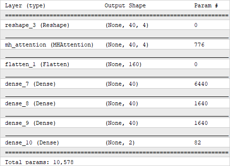
To build the initial model, we created a fairly simple architecture consisting of one attention layer, three fully connected hidden layers, and one fully connected output layer. We used almost the same model architecture above to build the convolutional model. The use of similar models enables the accurate evaluation of the impact of new solutions on the overall performance of the model.
heads=8
key_dimension=4
model5 = keras.Sequential([keras.layers.InputLayer(input_shape=inputs),
# Reformat the tensor into 3-dimensional. Specify 2 dimensions,
# as the 3rd dimension is determined by the size of the batch
# first dimension is for sequence elements
# second dimension is for the vector describing of one element
keras.layers.Reshape((-1,4)),
MHAttention(key_dimension,heads),
|
Since our attention layer returns a tensor of the same size as its input, we need to reshape the data into a two-dimensional space before using the block of fully connected layers.
# Reformat the tensor to 2-dimensional for fully connected layers
keras.layers.Flatten(),
keras.layers.Dense(40, activation=tf.nn.swish,
kernel_regularizer=keras.regularizers.l1_l2(l1=1e-7, l2=1e-5)),
keras.layers.Dense(40, activation=tf.nn.swish,
kernel_regularizer=keras.regularizers.l1_l2(l1=1e-7, l2=1e-5)),
keras.layers.Dense(40, activation=tf.nn.swish,
kernel_regularizer=keras.regularizers.l1_l2(l1=1e-7, l2=1e-5)),
keras.layers.Dense(targerts, activation=tf.nn.tanh)
])
|
It should be noted that despite the external similarity of the models, the model utilizing the attention mechanism layer uses five times fewer parameters.
However, using a single attention layer is a simplified model and is employed solely for comparative experimentation purposes. In practice, it's more common to use multiple consecutive attention layers. I suggest evaluating the impact of multiple attention layers used in the model on real-world data. To conduct such an experiment, we will sequentially add three more attention layers with the same parameters to our previous model.

Model using the Multi-Heads Self-Attention layer
model6 = keras.Sequential([keras.layers.InputLayer(input_shape=inputs),
# Reformat the tensor into 3-dimensional. Specify 2 dimensions,
# as the 3rd dimension is determined by the size of the package
# first dimension is for sequence elements
# second dimension is for the vector describing one element
keras.layers.Reshape((-1,4)),
MHAttention(key_dimension,heads),
MHAttention(key_dimension,heads),
MHAttention(key_dimension,heads),
MHAttention(key_dimension,heads),
# Reformat the tensor to 2-dimensional for fully connected layers
keras.layers.Flatten(),
keras.layers.Dense(40, activation=tf.nn.swish,
kernel_regularizer=keras.regularizers.l1_l2(l1=1e-7, l2=1e-5)),
keras.layers.Dense(40, activation=tf.nn.swish,
kernel_regularizer=keras.regularizers.l1_l2(l1=1e-7, l2=1e-5)),
keras.layers.Dense(40, activation=tf.nn.swish,
kernel_regularizer=keras.regularizers.l1_l2(l1=1e-7, l2=1e-5)),
keras.layers.Dense(targerts, activation=tf.nn.tanh)
])
|
We will compile all neural models with the same parameters: the Adam optimization method, standard deviation as the network error, and an additional accuracy metric.
model3.compile(optimizer='Adam',
loss='mean_squared_error',
metrics=['accuracy'])
|
We compiled neural network models with the same parameters as before.
Recurrent models are sensitive to the sequence of input signals provided. Therefore, when training a recurrent neural network, unlike the other models, you cannot shuffle the input data. Exactly for this purpose, when launching a recurrent model, we set the shuffle parameter to False. The convolution model and models using the attention layer have this parameter set to True. The remaining training parameters for the models remain unchanged, including the early stopping criterion when reaching a minimum error on the training dataset.
callback = tf.keras.callbacks.EarlyStopping(monitor='loss', patience=20)
history3 = model3.fit(train_data, train_target,
epochs=500, batch_size=1000,
callbacks=[callback],
verbose=2,
validation_split=0.01,
shuffle=True)
|
After slightly training the models, we visualize the results. We plot two graphs. On one of them, we will display the dynamics of error changes during the training and validation process.
# Plot the results of model training
plt.figure()
plt.plot(history3.history['loss'], label='Conv2D train')
plt.plot(history3.history['val_loss'], label='Conv2D validation')
plt.plot(history4.history['loss'], label='LSTM only train')
plt.plot(history4.history['val_loss'], label='LSTM only validation')
plt.plot(history5.history['loss'], label='MH Attention train')
plt.plot(history5.history['val_loss'], label='MH Attention validation')
plt.plot(history6.history['loss'], label='MH Attention 4 layers train')
plt.plot(history6.history['val_loss'], label='MH Attention 4 layers validation')
plt.ylabel('$MSE$ $loss$')
plt.xlabel('$Epochs$')
plt.title('Model training dynamics')
plt.legend(loc='upper right', ncol=2)
|
In the second graph, we plot similar results for Accuracy.
plt.figure()
plt.plot(history3.history['accuracy'], label='Conv2D train')
plt.plot(history3.history['val_accuracy'], label='Conv2D validation')
plt.plot(history4.history['accuracy'], label='LSTM only train')
plt.plot(history4.history['val_accuracy'], label='LSTM only validation')
plt.plot(history5.history['accuracy'], label='MH Attention train')
plt.plot(history5.history['val_accuracy'], label='MH Attention validation')
plt.plot(history6.history['accuracy'], label='MH Attention 4 layers train')
plt.plot(history6.history['val_accuracy'], label='MH Attention 4 layers validation')
plt.ylabel('$Accuracy$')
plt.xlabel('$Epochs$')
plt.title('Model training dynamics')
plt.legend(loc='lower right', ncol=2)
|
Then we will load the test dataset and evaluate the performance of the pretrained models on it.
# Load testing dataset
test_filename = os.path.join(path,'test_data.csv')
test = np.asarray( pd.read_table(test_filename,
sep=',',
header=None,
skipinitialspace=True,
encoding='utf-8',
float_precision='high',
dtype=np.float64,
low_memory=False))
|
# Split the test sample into input data and targets
test_data=test[:,0:inputs]
test_target=test[:,inputs:]
|
# Validation of model results on a test sample
test_loss3, test_acc3 = model3.evaluate(test_data, test_target, verbose=2)
test_loss4, test_acc4 = model4.evaluate(test_data, test_target, verbose=2)
test_loss5, test_acc5 = model5.evaluate(test_data, test_target, verbose=2)
test_loss6, test_acc6 = model6.evaluate(test_data, test_target, verbose=2)
|
The results of the model's performance on the test sample will be numerically logged and visualized on the graph.
# Output test results to the log
print('Conv2D model')
print('Test accuracy:', test_acc3)
print('Test loss:', test_loss3)
|
print('LSTM only model')
print('Test accuracy:', test_acc4)
print('Test loss:', test_loss4)
|
print('MH Attention model')
print('Test accuracy:', test_acc5)
print('Test loss:', test_loss5)
|
print('MH Attention 4l Model')
print('Test accuracy:', test_acc5)
print('Test loss:', test_loss5)
|
plt.figure()
plt.bar(['Conv2D','LSTM', 'MH Attention','MH Attention\n4 layers'],
[test_loss3,test_loss4,test_loss5,test_loss6])
plt.ylabel('$MSE$ $loss$')
plt.title('Test results')
|
plt.figure()
plt.bar(['Conv2D','LSTM', 'MH Attention','MH Attention\n4 layers'],
[test_acc3,test_acc4,test_acc5,test_acc6])
plt.ylabel('$Accuracy$')
plt.title('Test results')
plt.show()
|
We finalize our work on the Multi-Head Self-Attention mechanism. We have recreated this mechanism by means of MQL5 and in Python. In this section, we have prepared a Python script that creates a total of four neural network models:
- Convolution model
- Recurrent neural network
- Two models using Multi-Head Self-Attention technology
While running the script, we will conduct a brief training session for all four models using the same dataset. We will compare the performance of the trained models on the test dataset and analyze the results. This will allow us to compare the performance of various architectural solutions on real-world data. The test results will be provided in the next chapter.
