AIS Trade Channel Index MT5
- Indicators
- Aleksej Poljakov
- Version: 4.0
- Updated: 5 March 2021
- Activations: 5
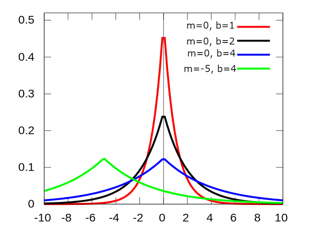
When analyzing financial time series, researchers most often make a preliminary assumption that prices are distributed according to the normal (Gaussian) law. This approach is due to the fact that a large number of real processes can be simulated using the normal distribution. Moreover, the calculation of the parameters of this distribution presents no great difficulties. However, when applied to financial markets, normal distribution does not always work. The returns on financial instruments often have a form that differs from normal. Too frequent and / or large emissions lead to the use of so-called "heavy tails" distributions. When constructing this indicator, we will assume that price levels are subject to the Laplace distribution. The main difference between this distribution is that it allows for a much wider range of values. Thanks to this, the Laplace distribution makes it possible to simulate price movements. In addition, the Laplace distribution is composite and therefore can be used in situations where low and high values occur under different conditions. Distribution itself In appearance, it differs significantly from normal. And the shape and location of the graph depends on two parameters - b and m.
Level setting
The main advantage of the Laplace distribution is the large range of argument values. So, when using the normal distribution, the majority of the values fall in the range from –3 to +3. And when using the Laplace distribution, the range expands to –5 ... + 5. Thus, it becomes possible to more accurately classify price changes and make more informed trading decisions. The approximate probability that the price will be within the specified limits is shown in the table.
| Range | Probability,% | Subrange | Probability,% |
|---|---|---|---|
| –1…+1 | 63,2 | 0…1 | 31,6 |
| –2…+2 | 86,5 | 1…2 | 11,6 |
| –3…+3 | 95,0 | 2…3 | 4,3 |
| –4…+4 | 98,2 | 3…4 | 1,6 |
| –5…+5 | 99,3 | 4…5 | 0,6 |
In general, the probability that the indicator value will reach the z value can be calculated using the formula:
Probability = (1-exp (- | z |)) * 100% / 2
And the boundaries of the range that correspond to a given probability can be calculated as follows:
Level = ± ln (1-Probability / 100), 0≤Probability <100
There are two types of levels that can be used for trading.
| Type I | Type II | ||
| Probability | Range | Probability | Range |
| 1/2 | ±0.693 | 2/3 | ±1.099 |
| 3/4 | ±1.386 | 8/9 | ±2.198 |
| 7/8 | ±2.079 | 26/27 | ±3.297 |
| 15/16 | ±2.772 | 80/81 | ±4.396 |
| 31/32 | ±3.466 | 242/243 | ±5.495 |
The first type of levels can be used as an additional filter as part of an existing trading strategy. The second type of levels can be used to make independent trading decisions.
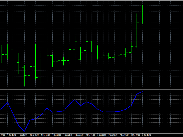
Interpreting Results
When using the indicator in trading, two basic rules apply:
- opening a Buy position with a negative value;
- opening a Sell position with a positive value.
It should be remembered that the further the indicator deviates from the zero line, the higher the probability of success.
Indicator setting
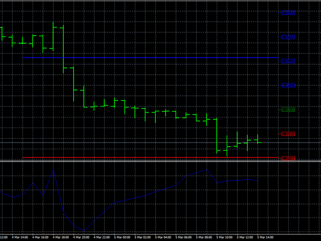
To configure the indicator, you need to set the values of the levels (you can use both the recommended ones and calculate them yourself).
Considering the specifics of calculations, iPeriod should be higher than 5.
The choice of the price constant depends on the trading strategy.

