Practical testing of convolutional models
Look at the amount of work we have already completed. This is something to be proud of. We have implemented three types of neural layers, which already allow us to solve some practical problems. Using those, we can create fully connected perceptrons of different complexity. Or we can create convolutional neural network models and compare the performance of the two models on the same set of source data.
Before assessing the practical capabilities of different neural network models, you should verify the correctness of the methods for error gradient propagation through the convolutional neural network. We have already performed such a procedure for fully connected neural layers in the section Checking the correctness of the gradient distribution.
Let me remind you of the essence of the procedure. The error gradient is a number that determines the slope of the tangent line to the function graph at the current point. It demonstrates how the value of a function will change when the parameter changes.
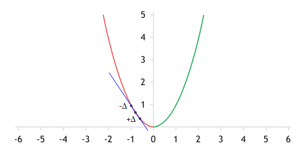
In geometry terms, the gradient is the slope of the tangent to the graph of the function at the current point
Of course, we are dealing with non-linear functions, and analytically computed error gradients provide only an approximate value. But when using a sufficiently small parameter change step, such an error becomes minimal.
Moreover, we can always determine how the function value changes when we experimentally alter a single parameter: we can take our function, change only one parameter, and calculate the new value. The difference between the two values of the function will show the influence of the analyzed parameter on the overall result at the current point.
Certainly, as the number of parameters increases, so do the costs of evaluating the influence of each parameter on the overall result. Therefore, neglecting a small error, everyone uses the analytical method to determine the error gradient. At the same time, by using the experimental method, we can assess the accuracy of our implemented analytical algorithm and adjust its operation if necessary.
When comparing the results of analytical and experimental methods for determining the error gradients, one point should be taken into account. To draw a straight line in a plane, two points are required. But if we draw a straight line through the current and new point, then such a straight line will not be tangent to the graph of the function at the current point. Most likely it will be tangent at some point between the current and future position. Therefore, to construct a tangent to the graph of a function at the current point, you will need to increase and decrease the current value of the indicator by the same small amount and calculate the function's value at both points. Then the line will touch the function at the point we need, and the effect of the parameter on the value of the function will be its average between two deviations.
When analyzing error gradient deviations between methods in a fully connected layer, we created the script check_gradient_percp.mq5. Let's make a copy of the script named check_gradient_conv.mq5. In the resulting copy, we will only change the CreateNet function. In it, after the input data layer, we will add one convolutional layer and one pooling layer.
bool CreateNet(CNet &net)
|
The convolutional layer will consist of two filters. The size of the convolution window is equal to two, its step is set to one. The activation function is Swish. The optimization method doesn't matter, as at this stage we won't be training the neural network. The size of one filter is recalculated based on the size of the previous layer and the convolution parameters.
//--- Convolutional layer
|
After the convolutional neural layer, we place the pooling layer. For it, we will specify the windows equal to two and the step of one. We will specify the activation function AF_AVERAGE_POOLING, which corresponds to the calculation of the average value for each source data window.
//--- Pooling layer
|
Further, the script code remains unchanged.
We launch the prepared script in two modes: using OpenCL technology and without it. As a result of testing, we obtained quite decent results. In both cases, we received deviations in the 11th decimal place.

The results of checking deviations of the error gradient between the analytical and experimental methods of determination
Now that we are confident in the correctness of our neural layer classes, we can proceed to the construction and training of convolutional neural networks. First, we need to decide how we want to use convolution.
In our dataset, each candlestick is represented by several indicators. In particular, when creating a training sample for each candlestick, we identified four indicators:
- RSI
- MACD histogram
- MACD signal line
- Deviation between the signal line and MACD histogram
Each of you can conduct a series of tests yourselves and determine your approach to using convolutional models. To me, the most obvious are two use cases.
- We can use convolution to determine certain patterns from indicator values at the level of each candlestick. In this version, we define the number of patterns to be searched for as the number of convolution filters. At the output of the convolutional layer, we get the degree of similarity of each candlestick with the desired patterns.
- It should be remembered that a fully connected neural layer is a linear function. Only the activation feature adds non-linearity. Therefore, in general, neurons do not evaluate dependencies between elements of the source data, but instead learn to recognize patterns from the set of source data. Hence, each neuron evaluates the current pattern independently of past data.
But when analyzing time series, sometimes the dynamics of the change in an indicator is more important than its absolute value. We can use convolution to determine patterns in the dynamics of indicators. To do this, we need to slightly rearrange the indicators, lining up the values of each indicator in a row. For example, we can start by arranging all the RSI indicator values in the source data buffer. Then, we can place all the elements of the MACD histogram sequence, followed by the data of the signal line. We will complete the buffer with deviation data between the signal line and the MACD histogram. Of course, it would be more visual to arrange the data in a tabular form, where each row would represent the values of a separate indicator. But, unfortunately, only one-dimensional buffers are used in the OpenCL context. Therefore, we will use virtual partitioning of the buffer into blocks.
After arranging each indicator into a separate row, we can use convolution to identify patterns in sequential values of a single indicator. By doing so, we are essentially identifying trends within the analyzed data window. The number of convolutional layer filters will determine the number of trends to be recognized by the model.
Testing convolution within a single candlestick
To test the operation of convolutional neural network models, let's create a copy of the perceptron_test.mq5 script perceptron_test.mq5 with the name convolution_test.mq5. At the beginning of the script, as before, we specify the parameters for script operation.
As with checking the correctness of the gradient distribution, we only need to change the function for describing the architecture of the CreateLayersDesc model. In it, after the layer of initial data, we add convolutional and pooling neural layers.
bool CreateLayersDesc(CArrayObj &layers)
|
Please note that for the convolutional layer, in the count field of the layer description object, we indicate not the total number of neurons, but the number of elements in one filter. In the window_out field, we will specify the number of filters to use. In the window and step fields, we will specify the number of elements per bar. With these parameters, we will obtain non-overlapping convolution, and each filter will compare the state of indicators at each bar with a certain pattern. The activation function is set to Swish, and the optimization method is set to Adam. We will use this optimization method for all subsequent layers. Except, of course, the pooling, which does not contain a weight matrix.
//--- Convolutional layer
|
The convolutional layer is followed by the pooling layer. In this implementation, I used Max Pooling, i.e., selecting the maximum element within the input window. We are using a sliding window of two elements with a step of one element. With this set of parameters, the number of elements in one filter will decrease by one. We do not use the activation function for this layer. The number of filters is equal to the same parameter of the previous layer.
//--- Sub-sample layer
|
Next comes an array of hidden fully connected layers. We will create them in a loop with the same parameters. The number of hidden layers to be created is specified in the script parameters. All hidden layers will have the same number of elements, which is specified in the script parameters. We will use the activation function Swish, and the weight matrix parameter optimization method, Adam, as we did for the convolutional layer.
//--- Block of hidden fully connected layers
|
At the end of the neural network initialization function, we will specify the parameters of the output layer. It will, just like in the previously created perceptron models, contain two elements with a linear activation function. We will use the Adam optimization method which is used by all other neural layers.
//--- Results Layer
|
The rest of the script code remains unchanged.
According to the testing results, the convolutional neural network model exhibited a less smooth graph. On it, we observe a wave-like decrease in the value of the error function. But at the same time, after 1000 iterations of updating the weight matrix, we got a lower value of the loss function.
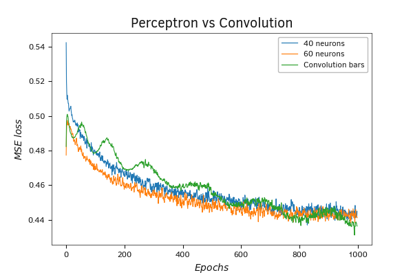
A comparative graph of the training progress of the perceptron and the convolutional neural network.
As the scale increases, we can also notice a tendency for the value of the loss function to potentially decrease with continued learning.
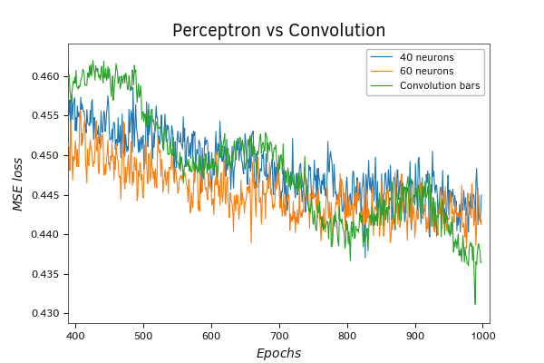
A comparative graph of the training progress of the perceptron and the convolutional neural network.
Testing of sliding window convolution by indicator values
Testing convolution with a sliding window on indicator values To experiment with finding patterns in the dynamics of indicator values, we need to make some modifications to the previously created script convolution_test.mq5. Let's create its copy with the name convolution_test2.mq5. We will make the first changes to the declaration of the convolutional layer. This time, we are creating a layer with a convolution window of three elements and a step of one element. With these parameters, the number of elements in one filter will be two less than the previous layer, but the total number of elements in the output buffer will increase by a factor equal to the number of filters used. The activation function and the optimization method remain unchanged.
//--- Convolutional layer
prev_count = descr.count = prev_count - 2;
|
In the pooling layer, the changes affected only the number of elements in one filter.
//--- Pooling layer
|
As mentioned before, for this test, we need to modify the sequence of source data being fed into the neural network. Therefore, we needed to make changes to the function of loading the training sample from the LoadTrainingData file.
As before, at the beginning of the function, we perform preparatory work. We declare instances of the necessary local objects and open the training dataset file for reading. The file name and path are specified in the function parameters. Let me remind you that the file with the training sample must be located within the sandbox of your terminal.
The result of the file opening procedure is checked by the received handle.
bool LoadTrainingData(string path, CArrayObj &data, CArrayObj &result)
|
After successfully opening the training sample file for reading, we start the loop of direct data loading. We will repeat the loop iterations until the file is finished. During each iteration, we will check if a command to close the program has been received before proceeding.
Inside the loop body, we will first prepare new instances of objects for loading patterns and target results.
//--- organize the loop to load training sample
|
We still use dynamic arrays to load data:
- data: array of source data patterns
- result: an array of patterns of target values for each pattern
- pattern: a buffer of elements of one pattern
- target: a buffer of target values of one pattern
However, to change the sequence of loaded data, we will first adjust the size of the pattern buffer matrix so that the first columns of the matrix correspond to the number of used indicators, and the rows correspond to the number of analyzed historical bars.
We create a system of nested loops. The outer loop has the number of iterations equal to the number of analyzed candles. The number of iterations in the inner loop is equal to the number of elements per candlestick. In the body of this looping system, we will write the initial data to the buffer matrix pattern. Since the data in the training sample file is in chronological order, we will write them in the same order. But as we read, we will distribute the information in the corresponding rows and columns of the matrix.
for(int i = 0; i < BarsToLine; i++)
|
After completing the iterations of the loop system, we only need to reformat the resulting matrix.
if(!pattern.Reshape(1, BarsToLine * NeuronsToBar))
|
The further process of loading the training sample has been moved without changes.
for(int i = 0; i < 2; i++)
|
As a result of training, such a neural network demonstrated an even greater amplitude of waves in the dynamics of loss function values. During the learning process, the amplitude of the waves was reduced. Such behavior could indicate the use of an elevated learning rate, the effect of which was mitigated by the Adam training method. I'd like to remind you that this training method utilizes an algorithm of individualized adaptation of the learning rate for each element of the weight matrix.
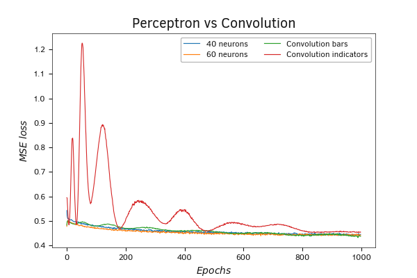
Comparative training graph of a perceptron and two convolutional neural network models
But back to the results of our test. Unfortunately, in this case, our model changes did not produce the desired reduction in model error. On the contrary, it has even increased. Nevertheless, there is hope for improved results when the learning rate is reduced.
Increasing the scale of the graph confirms the above conclusions.
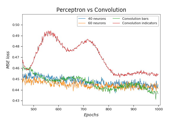
Comparative training graph of a perceptron and two convolutional neural network models
Combined model
We have examined the performance of two convolutional neural network models. In the first model, we carried out the convolution of indicator values within one candlestick. In the second model, we transposed (flipped) the original data and conducted a convolution in terms of indicator values. At the same time, in the first case, we carried out convolution of all indicators at once within one bar. I'd like to remind you that for each bar, we take four values from two indicators. In the second model, we used a convolution with a sliding window of three bars and a convolution window step of one bar. And here arises an obvious question: what results can be achieved if we combine both approaches? One more experiment will give us the answer to this question.
To conduct this test, we need to build another model. In practice, the creation of such a model did not take me much time. Let's discuss. In the first case, we took indicator values for each candlestick, while in the second case, we used three consecutive values (three consecutive bars) of each individual indicator. If we want to combine two approaches, then it would probably be logical to take all the values for three consecutive bars for convolution. In both approaches, we used a step of one bar. Therefore, we will keep this step.
To build such a model, we do not need to transpose the data. Therefore, we will build a new model based on the convolution_test.mq5 script. First, we will create a copy of it called convolution_test3.mq5. In it, we will change the parameters of the convolutional layer. In the training sample, the data is in chronological order, so the convolution window of the full three bars will be equal to 3 * NeuronsToBar. Then the step of the convolution window with the size of one bar will be equal to NeuronsToBar. With these parameters, the number of elements in one filter will be BarsToLine - 2. We leave the activation function and the parameter optimization method unchanged.
//--- Convolutional layer
|
The changes made to the parameters of the convolutional layer required a slight adjustment of the parameters of the pooling layer. Here we have only made changes to the number of elements in one filter.
//--- Pooling layer
|
The rest of the script code remains unchanged.
The training results of the new model turned out to be better than all the previous ones. The graph of loss function dynamics without amplitude waves lies slightly below the graphs of all previously conducted tests.
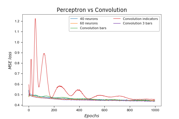
Comparative training graph of a perceptron and three models of convolutional neural networks
Increasing the scale of the graph confirms the above conclusions.
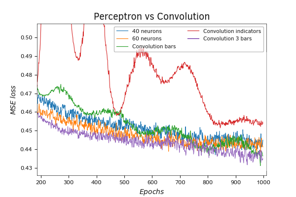
Comparative training graph of a perceptron and three models of convolutional neural networks
Testing Python models
In the previous section, we created a script with three neural network models in Python. The first perceptron model has three hidden layers, the second one has an additional Conv1D convolutional neural layer before the perceptron model, and in the third model, the Conv1D convolutional layer is replaced with Conv2D. At the same time, the number of parameters increased in each subsequent model. Based on the logic of our work, the models we created in Python should replicate the experiments conducted earlier with the neural network models built using MQL5. Therefore, the test results were fully expected and fully confirmed the earlier conclusions. For us, this is an additional confirmation of the correct operation of our library written in the MQL5 language. So, we can use it in our future work. Moreover, obtaining similar results when testing models that were entirely created using different tools eliminates the randomness of the results and minimizes the likelihood of making errors in the model creation process.
Let's get back to the test results. During the training process, the model with the Conv2D convolution layer showed the best results in reducing the error, which fully confirms the results obtained above. A significant gap between the error dynamics graphs of the training and validation sets in the case of the perceptron could indicate the underfitting of the neural network.
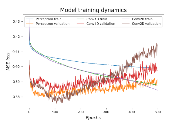
Comparative training graph of a perceptron and 2 models of convolutional neural networks (Python)
The error dynamics of the convolutional models are very close to each other. Their graphs are almost parallel. However, the model with the Conv2D convolutional layer shows less error throughout the training.
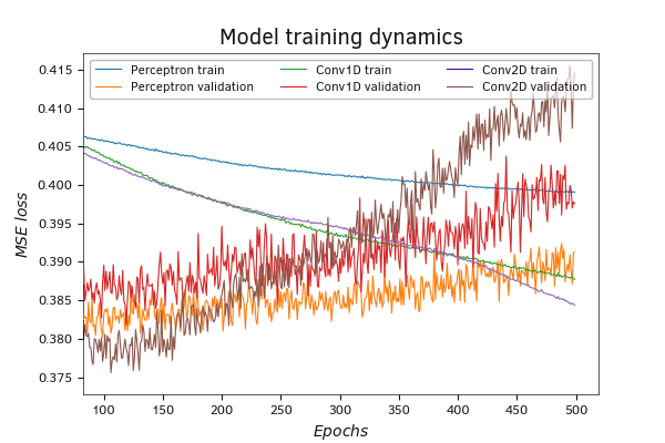
Comparative training graph of a perceptron and two convolutional neural network models (Python zoom)
On the validation set, the error graph of the Conv2D convolutional model first decreases, but after 100 epochs of training, there is an increase in the error. Along with a decrease in the error on the training set, this may indicate a tendency for models to overfit.
The graph of the Accuracy learning metric shows similar results.
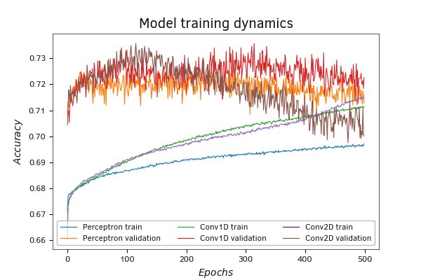
Comparative training graph of a perceptron and two convolutional neural network models (Python)
On the validation set, the graphs of all three models are closely intertwined in the range of 0.71—0.73. The graph shows the intersection of the training and validation sample graphs after 400.
I would like to remind you that the validation dataset is significantly smaller than the training dataset; it consists of the last patterns without shuffling the overall dataset. Hence, there's a high likelihood that not all possible patterns will be included in the validation dataset. In addition, the validation set can be influenced by local trends.
Checking the performance of all three trained models on the test set showed quite similar, albeit slightly contradictory, results.
Testing the mean squared error of the models revealed that the convolutional model with the Conv2D convolution layer achieved the best results. This model analyzes patterns within a single indicator using a sliding window convolution. During training, it performed the best among the tested models. Certainly, the differences in the performance metrics are not very significant, and it can be considered that all models showed similar results.
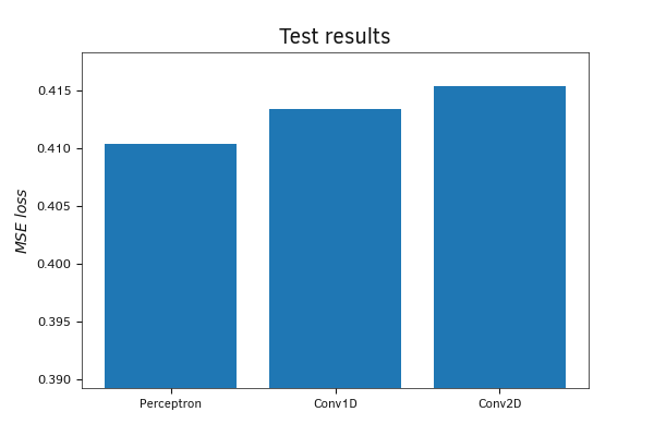
Comparison of model errors on a test set
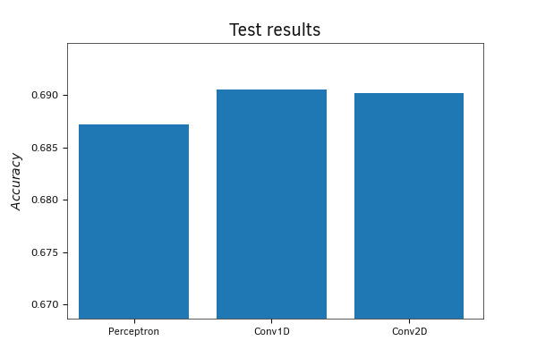
Comparison of the model accuracies on a test set
Comparison of the results by the Accuracy metric, in contrast to the just considered MSE graph, shows the best results for the Conv1D model. The model analyzes the patterns of each individual candlestick; the lowest result is for the perceptron. However, as with MSE, the gap between the results is small.
I suggest considering that all three models showed approximately equal results on the training dataset. The exact values of the metrics on the test sample are shown in the screenshot below.
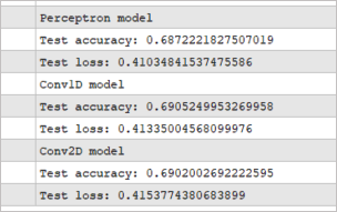
The exact values of model validation on the test set
Conclusions
According to the results of the tests, we can say:
- The models built using MQL5 during training demonstrate results similar to models built using the Keras library in Python. This fact confirms the correctness of the library we are creating. We can confidently continue our work.
- In general, convolutional models contribute to improving the performance of the model on the same training dataset.
- Approaches to convolution of the initial data may be different, and the results of the model may depend on the chosen approach.
- Combining different approaches within one model does not always improve the results of the model.
- Don't be afraid to experiment. When creating your own model, try different architectures and various data processing approaches.
In our tests, we used only one convolutional and one pooling layer. This can be referred to as an approach to building simple models. The most successful convolutional models used for practical tasks often employ multiple sets of convolutional and pooling layers. At the same time, the dimension of the convolution window and the number of filters change in each set. Like I said, don't be afraid to experiment. Only by comparing the performance of different models will you be able to choose the best architecture for solving your task.