Discussion of article "Application of the Eigen-Coordinates Method to Structural Analysis of Nonextensive Statistical Distributions"
Heh. Yes, such a peculiar "theory of everything".
I still see its value only from the fundamental point of view, in applied problems it is somehow more convenient to use approximations and special cases.
I still see its value only from the fundamental point of view, in applied problems it is somehow more convenient to use approximations and special cases.
Probably, it happened so because of the specific wrapping.
Themethod of eigen-coordinates was invented for "correct" solution of applied problems.
The paper [20] reveals this point in more detail:
i.e., "only with the fundamental" is better read as "including the fundamental".
And who is the author of this creation (article)? :-)
The author of this article is ready to answer your questions :)
The method of eigen-coordinates was developed by R,R. Nigmatullin:
[20] R. R. Nigmatullin, "Eigen-coordinates: New method of analytical functions identification in experimental measurements".
[21] R. R. Nigmatullin, "Recognition of nonextensive statistical distributions by the eigencoordinates method".
The decomposition of R(x) was published in [20], the decomposition of P1(x) and P2(x) in [21].
The mathematical justification of the method can be found in these articles.
Regarding the fundamental+applied problem - it would be interesting to check how good the q-Gaussian P2(x) and the Hilhorst and Scher solution P(U) are for describing real market data.
This would also require constructing the eigen-coordinates of P(U) by analogy with P2(x) (it has erf-1(x) in the argument, but the derivative and integral can be obtained analytically).
Once we have a differential equation for it, we can compare it with the structure of the equation for P2(x).
If P(U) is the limiting solution, it should work better on larger timeframes, this can be checked.
It is also desirable to improve the accuracy of the calculation of erf-1(x), the paper used a rational approximation, at some points |x-erf(erf-1(x))|~10^-5.
Regarding the fundamental+applied problem - it would be interesting to check how good the q-Gaussian P2(x) and the Hilhorst and Scher solution P(U) are for describing real market data.
This would also require constructing the eigen-coordinates of P(U) by analogy with P2(x) (it has erf-1(x) in the argument, but the derivative and integral can be obtained analytically).
Once we have a differential equation for it, we can compare it with the structure of the equation for P2(x).
If P(U) is the limiting solution, it should work better on larger timeframes, this can be checked.
It is also desirable to improve the accuracy of the erf-1(x) calculation, the paper used a rational approximation, at some points |x-erf(erf-1(x))|~10^-5.
Rumbas, rumbas, finger pointing :)
I am pleased with the appearance of this article, and also pleased that there are more and more articles that have a definite message.
.
To the point of the article.
My more than modest experience in the application of statistics shows that it is more important to be systematic in the application of statistical methods than to be in-depth in the use of individual methods.
From the article it is not clear:
1. what problem(s) of quotations this article solves.
2. what problem(s) of TS construction this article solves.
Without having such a review, it is difficult for me to judge about the practical value of this article.
Regarding the fundamental+applied problem - it would be interesting to check how good the q-Gaussian P2(x) and the Hilhorst and Scher solution P(U) are for describing real market data.
This would also require constructing the eigen-coordinates of P(U) by analogy with P2(x) (it has erf-1(x) in the argument, but the derivative and integral can be obtained analytically).
Once we have a differential equation for it, we can compare it with the structure of the equation for P2(x).
If P(U) is the limiting solution, it should work better on larger timeframes, this can be checked.
It would also be desirable to improve the accuracy of the erf-1(x) calculation, the paper used a rational approximation, at some points |x-erf(erf-1(x))|~10^-5.
This is probably the case because of the specific wrapper.
The method of eigen-coordinates was invented for "correct" solution of applied problems.
The paper [20] reveals this point in more detail:
i.e. "only with the fundamental" is better read as "including the fundamental".
My point in all this is this. Suppose we have some model, and on the basis of it we have obtained a theoretical function. And let it be that due to our ignorance we could not take into account some very insignificant but systematic factor. In this case, the method of eigen-coordinates because of its extraordinary sensitivity will give us a slap on the wrist, saying that the real data do not correspond to the model. But that's not true! - The model is correct, but it does not take into account only one factor, and from the practical point of view this deficiency may turn out to be insignificant at all (as in the same example of Hilhorst-Schell, where it is difficult to notice the difference even by eye). So, I would read "only from the fundamental" as "rather from the fundamental" in the sense that the value of maximum accuracy of correspondence may be not so essential from the applied point of view (for solving a practical problem), but from the fundamental point of view (thorough understanding of all the processes taking place).
In addition, the method only gives us a verdict that the model does not fit the experimental data, but does not tell us anything about the reasons for the discrepancy (as in my example - we cannot determine whether the model is "generally" correct with minor flaws or whether it should be completely revised), and this is a disadvantage.
- Free trading apps
- Over 8,000 signals for copying
- Economic news for exploring financial markets
You agree to website policy and terms of use
New article Application of the Eigen-Coordinates Method to Structural Analysis of Nonextensive Statistical Distributions is published:
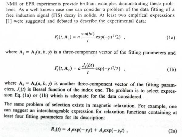
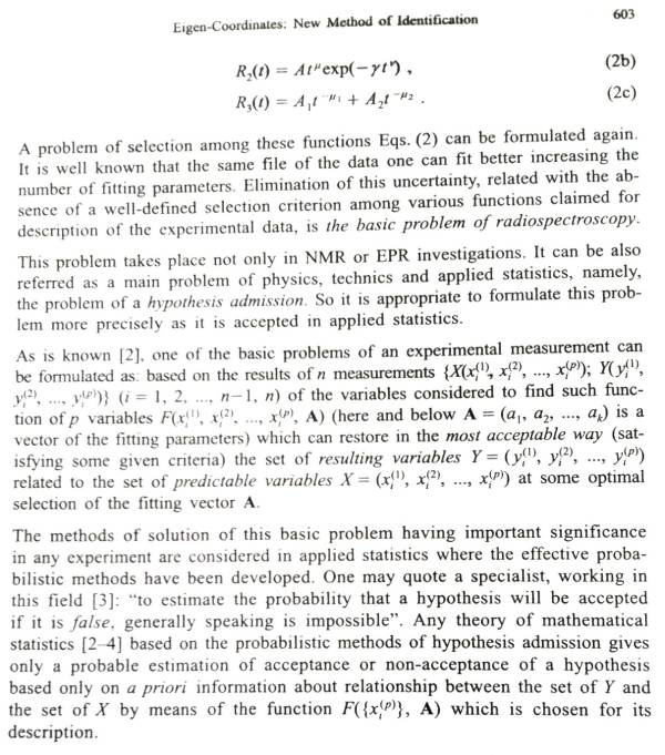
The major problem of applied statistics is the problem of accepting statistical hypotheses. It was long considered impossible to be solved. The situation has changed with the emergence of the eigen-coordinates method. It is a fine and powerful tool for a structural study of a signal allowing to see more than what is possible using methods of modern applied statistics. The article focuses on practical use of this method and sets forth programs in MQL5. It also deals with the problem of function identification using as an example the distribution introduced by Hilhorst and Schehr.
Author: MetaQuotes