Useful and exotic techniques for automated trading

Table of Contents

• Introduction
• Partial position closing algorithm, utilizing last bar movement
• Hybrid lot variation algorithm
• Averaging principle
• Direct and indirect signs of the consistency of a trading technique
• Using balance and equity waves
• Conclusion

Introduction

There are many trading techniques that the authors or the public think should be profitable. I will not consider these techniques in this article, since there is a lot of information about them on a wide variety of resources. I cannot offer anything new or interesting regarding these methods. Instead, I decided to create this article as a collection of several useful and non-standard techniques that would be useful both theoretically and practically. Some of these techniques may be familiar to you. I will try to cover the most interesting methods and will explain why they are worth using. Furthermore, I will show what these techniques are apt to in practice.

Partial position closing algorithm, utilizing last bar movement

Theory:

This approach may serve as a useful trading technique when we have opened a position and are not sure in which direction the price will move further. Smart partial position closing can compensate for losses from spreads, and even generate a profit following a good optimization.

Let us start with the following. Suppose we don't know where to exit, but we have already entered a position. It does not matter in which direction we have entered. Anyway, we will have to close the position sometime. Of course, some players can hold their positions for years. However, we assume that the robot should trade intensively and provide a high frequency of trades. It is possible to exit the entire volume or in a few steps, by closing the position partially. We know that the market has a flat structure, which means that the price tends to return to the position of the beginning of the current half-wave. In other words, an upward movement means that the probability of continuation is always less than 50%. Accordingly, the probability of an opposite movement is greater than 50%. If we close the entire position, we can miss all waves and miss profit, because we do not know the future amplitude of the waves. Partial closure can be helpful here. We will be able to take the maximum profit based on the fact that we do not know the nature of future waves.

Now that we know what waves are and that they will never disappear from the market, we can start with the position closing principle, which should provide the generation of at least some profit even if the entry is made incorrectly. Such a mechanism actually exists.

There can be many such algorithms, but I will show only one, which I believe to be the most efficient. It exploits the assumption that the larger and stronger was the move on the previous fully formed candlestick, the more likely it is that there will be a fairly strong rollback move. Generally speaking, what is the purpose of this mechanism? This is simple. The purpose is to increase profits while reducing losses. Impulses are actually waves too. But these waves are much more useful than the usual classical waves. The thing is that waves which are closest to the market are more reliable. The more powerful the impulse and the less its duration, the greater the probability of a rollback in the near future and the greater the magnitude of the expected rollback. The idea is to arrange the mechanism so that when the impulse power increases, the partial position closure would be stronger. I will show this in a picture:

Any function can be used to calculate the volume of the position part to be closed. I will show two of them. One is linear, and the second one is power:

• { D } - power
• { X } - previous bar movement in points
• { C } - scale factor
• { Lc(X) = C * Pow(X , D) } - a power function which calculates lot to be closed at the current candlestick
• { Lc(X) = C * X } - a linear function which calculates lot to be closed at the current candlestick

If you look closely, the linear function is just a special case of a power function for D = 1, so we can omit it as it is only an example for initial thinking logic. At the beginning thinking is always simple, but then, after thinking it over, we get much more versatile tools. It is only that you have to start with something simple.

To avoid the need to specify these coefficients directly and then care about their impact, we will introduce several control parameters that will determine these coefficients:

• { StartLotsToOnePoint } - close a position by this value when X = 1 (input parameter)
• { PointsForEndLots } - movement of the previous candlestick to the profit direction for the final position closing speed (input parameter)
• { EndLotsToOnePoint } - close the position by this value when X = PointsForEndLots  (input parameter)

Now let us compose a system of equations in order to calculate the coefficients and to obtain the final form of the function, expressed through the input parameters. For this purpose, the thoughts should be converted into mathematical expressions:

1. { Lc( 1 ) = StartLotsToOnePoint }
2. { Lc( PointsForEndLots ) = EndLotsToOnePoint }
   

So, all our equations are ready. Now we will write them in expanded form and will begin to solve the equations by gradually transforming them:

1. { C * Pow(1 , D) = StartLotsToOnePoint }
2. { C * Pow( PointsForEndLots  , D) = EndLotsToOnePoint }
   

In the first equation we can immediately find C, given that 1 in any degree is equal to itself:

• { C = StartLotsToOnePoint }

Dividing both sides of the second equation by "C" and then finding the logarithm of both sides of the equation to the base "PointsForEndLots", we get the following:

• { log( PointsForEndLots ) [ Pow( PointsForEndLots  , D)] = log( PointsForEndLots ) [  EndLotsToOnePoint / C ] }

Considering that the logarithm, where its base is the same logarithm raised to any power, is equal to this power, we can solve the equation with respect to the desired power:

• { D =  log( PointsForEndLots ) [  EndLotsToOnePoint / C ] }

We have found the second unknown coefficient. But this is not all, because MQL4 and MQL5 do not have a basic function implementing a logarithm to any required base, while there is only a natural algorithm. So, we need to replace the logarithm base by a natural logarithm (the natural algorithm is a logarithm to a base expressed by Euler's number). The absence of other logarithms in the language is not a problem, as any logarithm can be expressed in terms of the natural logarithm. This will be quite easy for anyone who understands at least something in mathematics. After changing the bas, the formula for our desired coefficient will look as follows:

• { D = ln(  EndLotsToOnePoint / C ) /  ln(  PointsForEndLots  ) }

Substitute the already known C coefficient and get:

• { D = ln(  EndLotsToOnePoint / StartLotsToOnePoint  ) /  ln(  PointsForEndLots  ) }

Now both coefficients can be substituted to the function template to obtain the final form:

• { Lc(X) = StartLotsToOnePoint  * Pow( X ,  ln(  EndLotsToOnePoint / StartLotsToOnePoint  ) /  ln(  PointsForEndLots  )  )  }
  

The advantage of this function is that the degree can be equal to one, or it can be greater than one, as well as less than one. Thereby it provides the maximum flexibility in adjusting to any market and trading instrument. If D = 1, we get a linear function. If D > 1, then the function is tuned to the assumption that all waves are scalable and the number of waves of a certain amplitude is inversely proportional to the amplitude (that is, if we count the number of waves, say on M5 and H1, in the same time period, it will turn out that there are 12 times less waves on H1, simply because there are 12 times less hourly candlesticks than five-minute candlesticks). If D < 1, we expect that we have more high-amplitude waves than small ones. If D > 1, we assume that there are mainly low-amplitude waves. 

Also note that you do not necessarily have to use a discretized price series as a sequence of bars - you can use ticks and any other preferred price segments. We use here bars simply because we have bars.

Code:

In the code, this function will look like this:

double CalcCloseLots(double orderlots0,double X)
   {
   double functionvalue;
   double correctedlots;
   if ( X < 0.0 ) return 0.0;
   functionvalue=StartLotsToOnePoint*MathPow(X ,MathLog(EndLotsToOnePoint/StartLotsToOnePoint)/MathLog(PointsForEndLots));
   correctedlots=GetLotAniError(functionvalue);
   if ( correctedlots > orderlots0 ) return orderlots0;
   else return correctedlots;
   }

The function that corrects the lot, so that lots take only the correct value, is highlighted in purple (there is no point in showing its insides). The function itself is calculated under the operator highlighted in green, but it is a part of a more general function which is called here:

void PartialCloseType()// close order partially
   {
   bool ord;
   double ValidLot;
   MqlTick TickS;
   SymbolInfoTick(_Symbol,TickS);
            
   for ( int i=0; i<OrdersTotal(); i++ )
      {
      ord=OrderSelect( i, SELECT_BY_POS, MODE_TRADES );
                            
      if ( ord && OrderMagicNumber() == MagicF && OrderSymbol() == _Symbol )
         {
         if ( OrderType() == OP_BUY )
            {
            ValidLot=CalcCloseLots(OrderLots(),(Open[0]-Open[1])/_Point);
            if ( ValidLot > 0.0 ) ord=OrderClose(OrderTicket(),ValidLot,TickS.bid,MathAbs(SlippageMaxClose),Green);
            }
         if ( OrderType() == OP_SELL )
            {
            ValidLot=CalcCloseLots(OrderLots(),(Open[1]-Open[0])/_Point);
            if ( ValidLot > 0.0 ) ord=OrderClose(OrderTicket(),ValidLot,TickS.ask,MathAbs(SlippageMaxClose),Red);
            }         
         break;
         }
      }

This code can be compiled in MQL5, because we use the MT4Orders library. Please note that these functions are suitable for testing. In order to use for real trading, you will need to carefully study them and refine them, taking care of errors and unaccounted cases. Anyway, the current version is quite suitable for testing in the strategy tester.

Testing the Expert Advisor:

To demonstrate how it works, I have created an EA version for MetaTrader 4, because when testing in MetaTrader 5, the spread will probably hide everything that we want to see. Instead, I set the spread to 1 and chose position opening in a random direction:

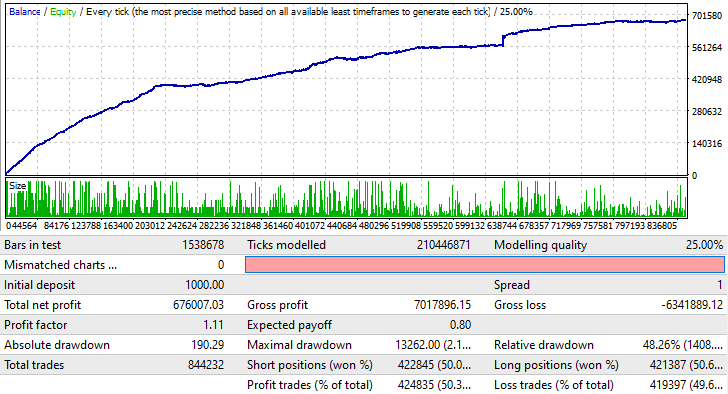
This also works in much the same way for other currency pairs. It can also work on higher timeframes, but this requires a little patience for finding appropriate settings. However, the test does not mean that you can immediately launch this EA on a real account. It only serves as a confirmation that this technique can be useful when utilized properly. Anyway, at this point this is very, very insufficient for profit even for this EA. But when combined with a good signal and a proper approach, this method can be profitable.

Hybrid lot variation algorithm

From the very beginning of market research, I was wondering how to shift the profit factor of any system towards positive values. This would mean that any strategy that does not depend so much on the spread, will obtain a very large advantage compared to any others, which have a profit factor close to one. Why exactly the profit factor needs to be improved? The answer is very simple: because both the relative drawdown of the entire system and the profitability of the system depend on this variable. Such a technique exists, and I will show it to you. But first, let us quickly go over the most famous trading techniques, which may utilize lot manipulation. There are the following alleged techniques for enhancing the profit factor:

• Martingale
• Reverse Martingale

In fact, it all boils down to two methods which are often discussed, but which can hardly bring anything but disappointment. It is all about a very simple mathematical principle, which I described in the article Grid and martingale: what are they and how to use them? It describes not the principles themselves, but what is common in all of them. The common thing is either a lot decrease or increase, depending on some conditions. If the conditions have nothing to do with the price formation nature, such a system is deliberately unprofitable.

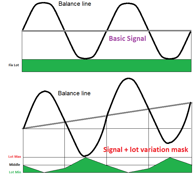
Any strategy which utilizes lot variation, has an underlying signal. We can get it by making so that lots for all orders are the same. This will help us understand if the underlying signal is in any way related to the price formation nature. In most cases, such a signal will produce zero mathematical expectation. But there is one parameter in this signal that can allow us to use both forward and reverse martingale at the same time. The required condition is the presence of a large number of low-amplitude waves. If you properly use the combination of a martingale and a reverse martingale, you can turn them into a hybrid mechanism which will turn a zero mathematical expectation into a positive one. The below figure shows how this may look like:

Theory:

Here we assume that we have a certain initial balance line, which, without taking into account the spread and commission, will always wander near the initial starting level, until one day you decide to stop trading with a positive or negative profit relative to the starting balance, or until the system slowly loses your deposit, which will be wasted by spreads, commissions and swaps. This means that any balance line of arbitrary trading is a somewhat wave process which fluctuates around the starting balance.

Based on this, we can divide the entire balance line into rising and falling sections (the figure shows a quarter of one full wave). If a wave quarter is growing, the lots should be decreased (reverse martingale); if the wave is falling, then the lots should be increased (martingale). The only obstacle to an endless lot increase is the fact that any account has a maximum allowable position volume. So, even if such a situation were possible, the deposit would not allow us to open extra positions. So, the lot should obviously fluctuate in a certain corridor of values and should not go beyond it. Therefore, the important point is that the amplitude of waves should not be too big, preferably more small waves and less large ones. If you look closely at the figure and at the lot variation mask below, you will understand how, using the hybrid variation, the line, relative to which the fluctuations occur, can acquire an upward slope, which is equivalent to a positive mathematical expectation and profit factor.

How to calculate lots in this case? The situation may seem unclear at first glance. Obviously, lots can reach one of the boundaries of our channel and never get out of there. For such a case we must provide a mechanism for returning to the starting lot, in order to obtain stable fluctuations around the average lot value. The obvious and only drawback of such a system is the intolerance of large amplitude waves. On a low-amplitude movement, the mechanism will perform perfectly. This problem is solved by a function which calculates the next lot in such a way that the function itself pushes the lots towards the middle, and the closer the lots of the previous closed order to one of the boundaries, the stronger the push. I will demonstrate this in the following figure:

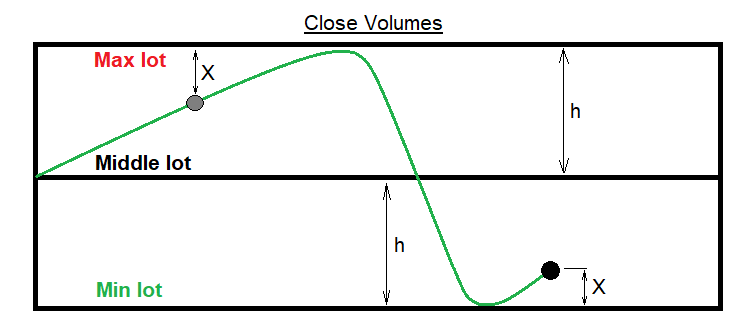
Now I will write a general view of a function which is suitable for this task, using the notation from the figure. But first, let us define the input parameters and auxiliary variables:

Input variables to control hybrid lot variation

• { MaxLot } - maximum lot corridor (input parameter)
• { MinLot } - minimum lot corridor (input parameter)
• { LotForMultiplier } - reference lot to increase or decrease the volume
• { ProfitForMultiplier } - loss and profit in points for the reference lot increase or decrease

Auxiliary variables

• { MiddleLot = (MaxLot + MinLot)/2 } - the middle between the maximum and minimum lot
• { h =  (MaxLot - MinLot)/2 } - half channel width (used for calculations)
• { L } - the lot of the last deal from the history
• { X } - auxiliary variable
• { OrderProfit , OrderComission , OrderSwap , OrderLots } - profit excluding commission, commission, calculated order swap, and the last order closing volume from the history (they are known)
• { TickSize } - an increase in the open position profit , provided that its volume is equal to 1 lot and the price has moved 1 point in the desired direction
• { PointsProfit = ( OrderProfit + OrderComission + OrderSwap ) / ( OrderLots * TickSize ) } - profit of the last order in history, converted into points

Function for the case when lots are above or below the center line

• { L  >=  MiddleLot  ?  X = MaxLot - L  } - if lots are in the upper part of the corridor, then the "X" value is the difference to the upper border of the channel
• { L  <  MiddleLot  ?  X = L - MinLot } - if lots are in the upper part of the corridor, then "X" is the distance to the lower channel border
• { L  >=  MiddleLot & PointsProfit < 0   ?  Lo(X) =  OrderLots - LotForMultiplier * (  PointsProfit / ProfitForMultiplier ) * ( X / h )  } - slowed lot increase when approaching the upper border of the channel
• { L  <  MiddleLot & PointsProfit >= 0   ?  Lo(X) =  OrderLots - LotForMultiplier * (  PointsProfit / ProfitForMultiplier ) * ( X / h )  } - slowed lot decrease when approaching the lower border of the channel
• { L  >=  MiddleLot & PointsProfit >= 0   ?  Lo(X) =  OrderLots - LotForMultiplier * (  PointsProfit / ProfitForMultiplier ) / ( X / h )  )  } - accelerated lot decrease 
• { L  <  MiddleLot & PointsProfit < 0   ?  Lo(X) =  OrderLots - LotForMultiplier * (  PointsProfit / ProfitForMultiplier ) / ( X / h )  } - accelerated lot increase

It is quite difficult to perceive all these relations, since they are hard to read. If you try to combine everything into a continuous function, you will get such a complex structure that it would be impossible to work with. I will show further how it looks like in the code, so everything will become clearer. Here I show the MQL4 style code implementation. The code can be easily run in MQL5 if you use the convenient and famous MT4Orders library:

Code:

double CalcMultiplierLot()
   {
   bool ord;
   double templot=(MaxLot+MinLot)/2.0;
   for ( int i=OrdersHistoryTotal()-1; i>=0; i-- )
      {
      ord=OrderSelect( i, SELECT_BY_POS, MODE_HISTORY );
      if ( ord && OrderSymbol() == CurrentSymbol &&  OrderMagicNumber() == MagicF )
         {
         double PointsProfit=(OrderProfit()+OrderCommission()+OrderSwap())/(OrderLots()*MarketInfo(CurrentSymbol,MODE_TICKVALUE));
         if ( OrderLots() >= (MaxLot+MinLot)/2.0 )
            {
            if ( PointsProfit < 0.0 ) templot=OrderLots()-(LotForMultiplier*(PointsProfit/ProfitForMultiplier))*((MaxLot-OrderLots())/((MaxLot-MinLot)/2.0));
            if ( PointsProfit > 0.0 ) templot=OrderLots()-(LotForMultiplier*(PointsProfit/ProfitForMultiplier))/((MaxLot-OrderLots())/((MaxLot-MinLot)/2.0)) ;
            if ( PointsProfit == 0.0 ) templot=OrderLots();
            break;
            }
         else
            {
            if ( PointsProfit > 0.0 ) templot=OrderLots()-(LotForMultiplier*(PointsProfit/ProfitForMultiplier))*((OrderLots()-MinLot)/((MaxLot-MinLot)/2.0));
            if ( PointsProfit < 0.0 ) templot=OrderLots()-(LotForMultiplier*(PointsProfit/ProfitForMultiplier))/((Orderlots()-MinLot)/((MaxLot-MinLot)/2.0));
            if ( PointsProfit == 0.0 ) templot=OrderLots();
            break;
            }
         }
      }
   if ( templot <= MinLot ) templot=(MaxLot+MinLot)/2.0;
   if ( templot >= MaxLot ) templot=(MaxLot+MinLot)/2.0;
         
   return templot;
   }

This library will be especially useful where you need to control each open order. So, this is the whole approach. The input variables of the algorithm are highlighted in yellow.

Testing the Expert Advisor:

This EA is also intended for MetaTrader 4, for the same reason as the previous EA, because it will be easier to see an improvement in the profit factor:

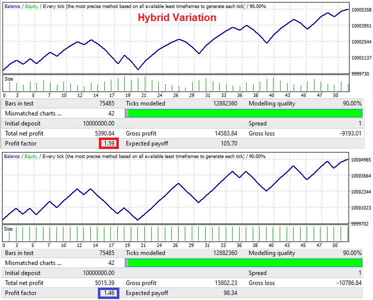
Signals in this Expert Advisor are generated in turn. Buying is followed by selling, and selling is followed by buying. This is done to demonstrate the essence of the mechanism. In the second test we use a fixed lot, and hybrid lot variation is used for the first test. It can be seen that the system can provide an improvement in the profit factor only if there are minimal balance fluctuations of the original signal. The system will not survive large waves.

Averaging principle

The averaging principle is a rather interesting algorithm. Although it is unprofitable, like the martingale grid and pyramiding, but it has one very interesting feature that can help in wave trading. If it is known that the movement will continue to a certain level and then there will necessarily be a roll back by a certain number of points, then averaging with martingale can be applied in this case. This technique works especially well with martingale, because martingale allows you to reduce the required rollback, while keeping the profit factor greater than 1.0. 

This principle exploits the assumption that if the price does not move in the direction of our open position, then, after some time, it will undoubtedly roll back by a part of this movement. But this does not always happen in reality, although you can fine-tune this algorithm for many symbols by studying the nature of its waves. In order to generate profit on this pullback, we need to predict it or determine it empirically.

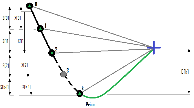
This also works with strong levels, because very often, when a level is broken out, the market may try to test it for inversion. If we guessed right with the direction of the first deal and the profit reached the required value, we close the deal and open a new one in the direction that seems more attractive. If the price has gone in the wrong direction, then, through certain steps, we can try to increase the volume of our position. We should be very carefully when increasing the position - it should be done precisely, based on the expected rollback. Below are the examples of two possible.

Example for a Buy series of orders:

Example for a Sell series of orders:

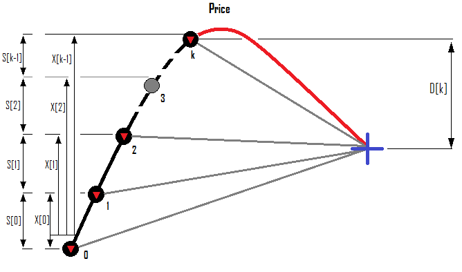
Now I will show how the profit or loss of all orders is calculated, and how, based on the existing situation, to calculate the lot of the next order, based on the required rollback. In order to close a fan of positions, it is necessary to know why this fan should be built and which condition makes it useful. I would use the Profit Factor. If the fan is positive, then its profit factor is also positive. It would be foolish to close the fan as soon as the total profit of all orders becomes positive, because any price fluctuation on the server or a slippage can shift the profit in the negative direction - such fans may seem useless under such conditions. In addition, the profit factor of the cycle provides an opportunity for the additional adjustment of the averaging aggressiveness, which can be used when optimizing an automated strategy or manually searching for settings.

Suppose that there is a limit on the maximum number of orders in a series. Then, suppose that we are in some unknown situation, where we have already opened k orders - their indices start from 0, as in any collections or arrays. So, the index of the last order in the series will be "k-1". When we open the next order, its index will be k and the number of orders will be "k + 1". Let us formalize these ideal into the input data of the problem:

• { MaxOrders } - the maximum allowable number of orders in a series
• {  k = 0 ... 1 ... 2 ...  (MaxOrders-1)  } - the index of the next order in the series, which we want to open if we do not generate profit from the previous approach
• {  ProfitFactorMax } - allowable profit factor for closing
• {  i = 1 ... 1 ... 2 ... k  } - indices of already existing orders of the fan and of the next order which we want to open
• {  S[i-1]  } - the distance in points from the previous order to the current one
• {  X[i-1]  } - the distance in points from the zero order of the series to the current one
• {  D[k]  } - predicted rollback in the desired direction relative to the open price of the last order of the series

Additionally, we can say that the MQL4 and MQL5 languages provide the following data when we refer to a specific order, which we need to describe all the calculation options:

• {  P[i] } - the profit of a specific order without excluding commission and swaps
• {  С[i] } - commission of the selected order
  
• {  S[i] } - calculated orders swaps during a rollover at 0:00
  
• {  L[i] } - order volume
  
• {  Sp[i] } - spread when opening a Buy position / current spread for Sell positions
• { TickSize } - an increase in the open position profit , provided that its volume is equal to 1 lot and the price has moved 1 point in the desired direction

Not all of these values will be needed for practical use in automated trading, but they allow highlighting of all possible options for calculating these values. Some of these values, which are relevant and can be depicted in relation to the price, are shown in the above figures. Let us start with the simplest calculation method that I use in my code:

If the first order closes with positive result, then do nothing. At any moment that we consider appropriate, we open a new order in the desired direction. If the price has not reached the target and has gone in the opposite direction, then we must decide how many points the price should move in the loss-making direction in order to open the next order (S[k-one] ). If the price has reached this level, then we must decide which rollback is appropriate (D [k]). After that, we must determine the lot of the order, which we will open now so that, with a planned rollback, we get the required profit factor of all orders greater than the value we have chosen (ProfitFactorMax). To do this, we first need to calculate which profit will be generated by currently open orders, as well as which loss will be generated, and their total value. I will explain the purpose of this later, after writing the corresponding formulas:

First, let us introduce the future profit value for each specific order. It is equal to the current profit and the increment that the order will receive, provided that the required rollback will happen:

• {  j = 0 ... 1 ... 2 ... k-1 }
  
• {  PF[j] = P[j] + С[j] + S[j] + (D[k] * L[j] * TickSize) } - the profit of a specific order will be equal to this value when the required rollback happens
• {  PF[k] = { ( D[k] - Spread[k] ) * L[k] * TickSize } - this value cannot be calculated as it contains the required lot of the position which we want to open; but this expression will be needed later
  

In the first case the P[i] value is known, and we can obtain it using the built-in language functions, as well as we can calculate it ourselves. This calculation method will be shown at the end of the article as an addition, because everything can be found by using standard language means. As for the last order in the series which we are going to open, it also needs a commission and swap, but these values can only be obtained for already open orders. Furthermore, it is impossible to determine the swap value as we do not know if the position will switch through 0:00. There will always be inaccurate values. It is possible to select only those currency pairs which have positive swaps 

After that we can use this predicted profit to split profitable and losing orders and to calculate the resulting profit factor:

• {  i = 0 ... 1 ... 2 ... k } - indices of already open orders
• {  Pr[i] >= 0, Ls[i]  >= 0 } - introduce 2 arrays which will accept order profit or loss depending on its sign ("+" will be used for profit, which is required for calculating the profit factor)
• {  PF [i] < 0  ?  Pr[i] = 0 & Ls[i] = - PF[i]  } - if the order profit is negative, then write its profit as "0", while the profit value should be written with an inverted sign into a variable for losses
• {  PF [i] > 0 ?  Ls[i] = 0 & Pr[i] = PF[i]  } - if the order profit is positive, simply write it to the appropriate array and set a zero value in the loss array
  

After filling these arrays, we can write a formula to calculate the total profit and loss, as well as their result.

• { SummProfit = Summ[0,k]( PF[i] ) } - total profit module of all profitable orders
• { SummLoss = Summ[0,k]( Ls [i] ) } - total loss module of all losing orders
  

Now we need to write the loop closing condition:

• { SummLoss > 0 ?  SummProfit/SummLoss  = ProfitFactorMax }

To use this equation further, you need to understand that the profit of the last order in the series is always positive when a positions fan is closed. Based on this, you can write:

• { SummProfit = Summ[0,k-1]( PF[j] )  +  PF[k] }
  

Substitute this value into the equation and get the following:

• {  ( Summ[0,k-1]( PF[j] )  +  PF[k] ) /  SummLoss  =  ProfitFactorMax }
  

Now, by solving this equation for PF[k], we get:

• { PF[k]  =  ProfitFactorMax * SummLoss  -  Summ[0,k-1]( PF[j] ) }
  

Considering that we already have a formula for the PF[k] value, we can substitute this expression here and get:

• { ( D[k] - Spread[k] ) * L[k] * TickSize = ProfitFactorMax * SummLoss  -  Summ[0,k-1]( PF[j] ) }
  

Now we can solve this equation with respect to L[k]. Thus, we will finally get the formula for calculating the required position volume to open:

• { L[k] =  ( ProfitFactorMax * SummLoss  -  Summ[0,k-1]( PF[j] ) )  /  ( ( D[k] - Spread[k] ) *  TickSize ) }
  

That is all. Now let us consider how to calculate the P[i] value without using built-in functions.

• { P[i] = ( X[i-1] - Spread[i] ) * L[i] * TickSize + С[j] + S[j] }
  

Calculating the rollback value

Now let us look at rollback calculation methods. I use two ways. There can be a lot of them, but I will provide only two methods which I think the most useful. The rollback is calculated in relation to how much the price has gone in the wrong direction. This means that D[i] and X[i] can be connected by any function which is positive on the entire positive X axis:

• { D=D(X) }
• { D[k] = D( X[k-1] ) }

I use two functions for calculating the rollback. The first one is linear. The second one is a power function. The second function is more difficult, but more interesting. Here are the functions:

• { D = K * X }
• { D = DMin + C * Pow(S , X) }

The coefficients to be found are highlighted. Based on these coefficients, the functions begin to act differently and, accordingly, we can flexibly adjust our strategy to a specific currency pair or timeframe.

1. { K } - rollback coefficient for a linear function (it is also used as an input parameter for an automated system) 
   
2. { DMin } - the minimum allowed rollback (D >= DMin, in the case of a power function)
   
3. { C } - power function scaling factor
4. { S } - the base of the exponentiation

Strictly speaking, C can be added to the degree, but I think in this form the function is more readable and convenient to use. Also note that the values K and DMin are input parameters, so these coefficients are already known to us. It is not clear how to calculate the two remaining coefficients. Let us do it now. In order to find 2 unknown values, we need a system of at least two equations. The coefficients can be found by solving the system. in order to write such a system, we first need to decide how the function form will be controlled. In fact, I have chosen the current form of the power function because it would be easier and more convenient to make a smooth decrease in the rollback. That is why I have chosen the power function. The considerations were as follows:

1. { HalfX } - price movement for the half of the additional rollback (an additional input parameter to control the function)
2. { D(0) = DMin + K*DMin }
3. { D(HalfX) = DMin + K*DMin/2 }

Thus, we get the required system of equations, which we will solve. In other words, we set the price movement towards loss, relative to the first open order, in which the addition to the rollback is half the value at the start. This addition has a maximum value at the start. As a result, we get a function which cannot take a value less than the minimum rollback, and as X tends to infinity, the function to the minimum rollback. Mathematically, it is expressed as follows:

• { D >= DMin }
  
• { Lim( X -> +infinity ) = DMin }

Now we can start solving this system of equations, but first let us rewrite the full system:

1. { DMin + C * Pow(S , 0) = DMin + K*DMin } 
2. { DMin + C * Pow(S , HalfX) =  DMin + K*DMin/2 }

In the first equation, we can immediately find C, considering the fact that any number in the zero power turns into one. Thus, we exclude the S variable. All we need to do now is solve the equation relative to the C variable. 

• { С = K * DMin }
  

Now that we have C, we can find the remaining unknown S by simply substituting the previous expression for the C variable:

• { Pow(S , HalfX) = 0.5 }

In order to eliminate the degree, we should raise both parts of the equation to the degree reciprocal of HalfX. As a result, we will obtain the following simple expression which will be the desired coefficient:

• { S = Pow(0.5  , 1/HalfX) }

Now we can write our power function by substituting the coefficients. This describes everything we need to implement this strategy:

• { D(X) = DMin + K *  DMin * Pow( Pow(0.5  , 1/HalfX)  , X ) }

This is how this function will look in the code:

Code:

double D(double D0,double K0,double H0,double X)
   {
   return D0+(D0*K0)*MathPow(MathPow(0.5,1.0/H0),X);
   }

Here are a few more important functions that will be used in the EA to test the theory. The first one is the function that determines the distance in points from the price to the nearest open order in the series:

double CalculateTranslation()
   {
   bool ord;
   bool bStartDirection;
   bool bFind;
   double ExtremumPrice=0.0;
   
   for ( int i=0; i<OrdersTotal(); i++ )
      {
      ord=OrderSelect( i, SELECT_BY_POS, MODE_TRADES );
      if ( ord && OrderMagicNumber() == MagicF && OrderSymbol() == Symbol() )
         {
         if ( OrderType() == OP_SELL ) bStartDirection=false;
         if ( OrderType() == OP_BUY ) bStartDirection=true;
         ExtremumPrice=OrderOpenPrice();
         bFind=true;
         break;
         }
      }      
   for ( int i=0; i<OrdersTotal(); i++ )
      {
      ord=OrderSelect( i, SELECT_BY_POS, MODE_TRADES );
                        
      if ( ord && OrderMagicNumber() == MagicF && OrderSymbol() == Symbol() )
         {
         if ( OrderType() == OP_SELL && OrderOpenPrice() > ExtremumPrice ) ExtremumPrice=OrderOpenPrice();
         if ( OrderType() == OP_BUY && OrderOpenPrice() < ExtremumPrice ) ExtremumPrice=OrderOpenPrice();
         }
      }
   if ( bFind )
      {
      if ( bStartDirection ) return (ExtremumPrice-Close[0])/_Point;
      else return (Close[0]-ExtremumPrice)/_Point;      
      }   
   else return -1.0;
   }

We need this function in order to comply with the required step between orders in the series. This step will be fixed. Do not forget that the "Close[]" array is not implemented in MQL5 and we need to implement it as it was shown in my previous articles. I think this step is quite clear.

In order to calculate the current X and D, we will use the following function, which does not have return values, like all further functions. It will write the result to global variables (it is better to minimize access to orders and avoid unnecessary calls of the functions working with the history:

double Xx;//shift of X
double Dd;//desired rollback of D
void CalcXD()//calculate current X and D
   {
   bool ord;
   bool bStartDirection=false;
   bool bFind=false;
   double ExtremumPrice=0.0;
   
   for ( int i=0; i<OrdersTotal(); i++ )
      {
      ord=OrderSelect( i, SELECT_BY_POS, MODE_TRADES );
      if ( ord && OrderMagicNumber() == MagicF && OrderSymbol() == Symbol() )
         {
         if ( OrderType() == OP_SELL ) bStartDirection=false;
         if ( OrderType() == OP_BUY ) bStartDirection=true;
         ExtremumPrice=OrderOpenPrice();
         bFind=true;
         break;
         }
      }   
   
   for ( int i=0; i<OrdersTotal(); i++ )
      {
      ord=OrderSelect( i, SELECT_BY_POS, MODE_TRADES );
                        
      if ( OrderMagicNumber() == MagicF && OrderSymbol() == Symbol() )
         {
         if ( OrderType() == OP_SELL && OrderOpenPrice() < ExtremumPrice ) ExtremumPrice=OrderOpenPrice();
         if ( OrderType() == OP_BUY && OrderOpenPrice() > ExtremumPrice ) ExtremumPrice=OrderOpenPrice();
         }
      }
   Xx=0.0;
   Dd=0.0;   
   if ( bFind )
      {
      if ( !bStartDirection ) Xx=(Close[0]-ExtremumPrice)/_Point;
      if ( bStartDirection ) Xx=(ExtremumPrice-Close[0])/_Point;
      if ( MODEE==MODE_SINGULARITY ) Dd=D(DE,KE,XE,Xx);
      else Dd=Xx*KE;
      }      
   }

This code is fully compatible with the MT4Orders library and thus it can be compiled in MQL5. This also refers to the functions that will be discussed further. The input variables of the algorithm are highlighted in yellow.

To calculate the current and predicted profit we will use three variables:

double TotalProfitPoints=0.0;   
double TotalProfit=0;
double TotalLoss=0;   

Return values will be added to these variables, while the functions themselves will have no return values - this we avoid order iterations every time, which slows down the code operation several times.

One of the next two functions will be used for the closing condition, and the second one will be used for calculating the predicted profit of currently open positions:

void CalcLP()//calculate losses and profits of all open orders
   {
   bool ord;
   double TempProfit=0.0;
   TotalProfit=0.0;   
   TotalLoss=0.0;    
   TotalProfitPoints=0.0;
   
   for ( int i=0; i<OrdersTotal(); i++ )
      {
      ord=OrderSelect( i, SELECT_BY_POS, MODE_TRADES );
                            
      if ( ord && OrderMagicNumber() == MagicF && OrderSymbol() == Symbol() )
         {
         TempProfit=OrderProfit()+OrderCommission()+OrderSwap();
         TotalProfitPoints+=(OrderProfit()+OrderCommission()+OrderSwap())/(OrderLots()*SymbolInfoDouble(Symbol(),SYMBOL_TRADE_TICK_VALUE));
         if ( TempProfit >= 0.0 ) TotalProfit+=TempProfit;
         else TotalLoss-=TempProfit;
         }
      }
   }
   
void CalcLPFuture()//calculate losses and profits of all existing orders in the future
   {
   bool ord;
   double TempProfit=0;
   TotalProfit=0;   
   TotalLoss=0;    
    
   for ( int i=0; i<OrdersTotal(); i++ )
      {
      ord=OrderSelect( i, SELECT_BY_POS, MODE_TRADES );
                            
      if ( ord && OrderMagicNumber() == MagicF && OrderSymbol() == Symbol() )
         {
         TempProfit=OrderProfit()+OrderCommission()+OrderSwap()+(OrderLots()*SymbolInfoDouble(Symbol(),SYMBOL_TRADE_TICK_VALUE)*Dd);
         if ( TempProfit >= 0.0 ) TotalProfit+=TempProfit;
         else TotalLoss-=TempProfit;
         }
      }
   }

Also, here is the predicate function for the order series closing condition:

bool bClose()
   {
   CalcLP();
   if ( TotalLoss != 0.0 && TotalProfit/TotalLoss >= ProfitFactorMin ) return true;
   if ( TotalLoss == 0.0 && TotalProfitPoints >= DE*KE ) return true;
   return false;
   }

Testing the Expert Advisor:

I have created an expert advisor for MetaTrader 5 using the described principle, as this method, when applied properly, can overcome almost any spreads, commissions and swaps. Here is the testing result of the EA exploiting averaging:

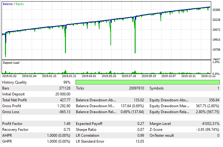
However, please note that it is only a trading technique which must be used very carefully. Nevertheless, it is very flexible and can be used in tandem with a wide variety of strategies. Again, please be careful.

Direct and indirect signs of the consistency of a trading technique

Within the framework of this article, it would be useful to consider which mathematical backtest variables can prove that the used technique strengthens our strategy or even turns a losing strategy into a profitable one. The question is very important, because if we interpret the backtest results incorrectly, we can exclude an actually working technique or utilize a wrong one. When developing new trading techniques, I always follow two rules, which create a necessary and sufficient condition for the most probable detection of working techniques and the most probable rejection of false ones:

1. The size of the data sample, as well as the number of trades in the backtest, should be maximized for statistical evaluation
2. Even a slight change in backtest values can indicate positive changes

In many cases, any positive change can be amplified to make it beneficial for trading. There are undeniable advantages:

1. Such trading techniques can work on any trading instrument
2. Techniques can be combined and turned into hybrids
3. When used correctly, your chances of generating a profit are greater than of having a loss, even with a spread

Now I will show which variables should be analyzed when trying to use a trading technique. Let us use the example of the last trading technique discussed in this article. Let us start with backtest metrics and see how to use them to create synthetic metrics to detect improvements.

First of all, pay attention to the following variables:

• Final backtest profit
• Maximum balance drawdown
• Maximum equity drawdown

There are some additional, more accurate variables which could help, but which are not available in the strategy tester reports:

• Average balance drawdown
• Average equity drawdown

Why do these metrics show accurately how safe and profitable the system is? The point is that for any backtest, there are the following mathematical identities, like for any trading system that trades on a demo or real account:

• { i = 0 ... 1 ... 2 ... m } - the number of a half-wave (a half-wave is one growing equity or balance segment, followed by a falling one)
• { j = 0 ... 1 ... 2 ... k } - negative half-wave segments (balance segments begin and end at the position opening and closing point, and equity segments end and begin at other points)
• { OrderProfit[j]-OrderComission[j]-OrderSwap[j] < 0 !  Lim( m --> +infinity ) [ Summ(i) [Summ(j) [ OrderProfit[j]-OrderComission[j]-OrderSwap[j] ]] / m  ] = total profit excluding commission spreads and swaps   } - average drawdown for backtest or trade balance
• { SegmentEquity[j]-SegmentComission[j]-SegmentSwap[j] < 0 !  Lim( m --> +infinity ) [ Summ(i) [Summ(j) [ SegmentEquity[j]-SegmentComission[j]-SegmentSwap[j] ]] / m  ] = total profit excluding commission spreads and swaps      } - average drawdown for backtest or trade balance

In other words, the average drawdown, both in terms of balance and equity, with an endless backtest or endless use of the strategy on a demo or real account, tends to the value of the final balance, if the transaction fee were zero. Of course, this is true only when the strategy has a pronounced positive profit. If the total profit has a negative sign, you can try mirror formulas, in which you should sum up not negative segments, but positive ones. But it is most convenient to operate with an already known positive backtest and to apply some techniques to it. This however does not mean that a global backtest will show profit. You should find such history intervals where the strategy shows profit (preferably several such intervals). Then apply an approach. 

Let us see now how, using a simple martingale, we can strengthen its stability and slightly shift its performance towards profit. Based on the formulas given above, it is possible to draw up such synthetic metrics, according to which it is possible to evaluate the effect of the trading technique on trading as a whole, based on a few small segments:

Input data for synthetic metrics:

• { Tp } - final backtest or trading profit
• { BdM } -  average balance drawdown
• { EdM } - average equity drawdown
• { BdMax } - maximum balance drawdown
• { EdMax } - maximum equity drawdown

The color highlights the data not available from the backtest. But this data can be calculated in the code and displayed at the end of trading or backtest. But I prefer to use other data that is available. The point is that the smaller the average drawdown, the smaller the maximum drawdown from both values in most cases. These values are very closely tied to probabilities, and changes in one metric usually entail approximately proportional changes in another metric. 

Synthetic metrics:

• { A = Tp/BdM } - equal to one if the strategy does not predict the future, and more than one if it knows how to predict and earns (which is equivalent to answering the question about its profitability)
• { B = Tp/EdM } - the same as the previous value
• { C = Tp / BdMax } - if there is an increase in this metric, then we can conclude that the technique increases the effectiveness of the method (a decrease means the negative effect)
• { D = Tp / EdMax } - the same as the previous value

Any of these 4 criteria can be used. The first two of them are more accurate, but the backtest cannot provide the necessary data to calculate them, so you would have to read the input data. The other two can be calculated by using values from the backtest. So, I personally use the last two metrics, because they are available and can be easily found. Now, let us view the application of this method using an example of a simple martingale that closes by stop orders. We will try to strengthen its variables using the last exotic approach.

Using balance and equity waves

Theory:

In fact, this technique can be used not only for martingale, but also for any other strategies that have a sufficiently high trading frequency. In this example, I will use the metric based on the balance drawdown. Because everything related to balance is considered easier. Let us divide the balance chart into rising and falling segments. Two adjacent segments form a half-wave. The number of half-waves tends to infinity as the number of transactions tends to infinity. A finite sample will be enough for us to make the martingale a little more profitable. The following diagram explains the idea:

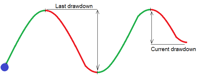
The figure shows a formed half-wave and the one that has just begun. Any balance graph consists of such half-waves. The size of these half-waves constantly fluctuates, and we can always distinguish groups of such half-waves on the chart. The size of these half-waves is smaller in one wave and is larger in the other. So, by gradually lowering the lots, we can wait until a half-wave with a critical drawdown appears in the current group. Since the lots of this critical drawdown will be minimal in the series, this will increase the overall average metrics of all groups of waves and, as a result, the same performance variables of the original test should also increase.

For implementation, we need two additional input parameters for the martingale:

• { DealsMinusToBreak } - the number of losing trades for the previous cycle, reaching which the starting lot of the cycle should be reset to the starting value
• { LotDecrease } - step for decreasing the starting lot of the cycle when a new cycle appears in the history of trades

These two parameters will allow us to provide increased lots for safe half-wave groups and reduced lots for dangerous half-wave groups, which should, in theory, increase the above mentioned performance metrics.

The following code will be added to the martingale EA. It calculates the starting lot of the next cycle and resets it if necessary:

Code:

double DecreasedLot=Lot;//lot to decrease
double CalcSmartLot()//calculate previous cycle
   {
   bool ord;
   int PrevCycleDeals=0;
   HistorySelect(TimeCurrent()-HistoryDaysLoadI*86400,TimeCurrent());
   for ( int i=HistoryDealsTotal()-1; i>=0; i-- )
      {
      ulong ticket=HistoryDealGetTicket(i);
      ord=HistoryDealSelect(ticket);
      if ( ord && HistoryDealGetString(ticket,DEAL_SYMBOL) == _Symbol 
      && HistoryDealGetInteger(ticket,DEAL_MAGIC) == MagicC 
      && HistoryDealGetInteger(ticket,DEAL_ENTRY) == DEAL_ENTRY_OUT )
         {
         if ( HistoryDealGetDouble(ticket,DEAL_PROFIT) > 0 )
            {
            for ( int j=i+1; j>=0; j-- )//found a profitable deal followed by losing (count them)
                {
                ticket=HistoryDealGetTicket(j);
                ord=HistoryDealSelect(ticket);
                if ( ord && HistoryDealGetString(ticket,DEAL_SYMBOL) == _Symbol 
                && HistoryDealGetInteger(ticket,DEAL_MAGIC) == MagicC 
                && HistoryDealGetInteger(ticket,DEAL_ENTRY) == DEAL_ENTRY_OUT )
                   {
                   if ( HistoryDealGetDouble(ticket,DEAL_PROFIT) < 0 )
                      {
                      PrevCycleDeals++;
                      }
                   else
                      {
                      break;
                      }
                   }                
                }
            break;    
            }
         else
            {
            break;
            }
         }
      }
      
   if ( PrevCycleDeals < DealsMinusToBreak ) DecreasedLot-=LotDecrease;
   else DecreasedLot=Lot;
   if ( DecreasedLot <= 0.0 ) DecreasedLot=SymbolInfoDouble(_Symbol,SYMBOL_VOLUME_MIN);

   return DecreasedLot;
   }

Input parameters are highlighted in yellow. Please note that this is a tests function, which is only suitable in this form for testing in the Strategy Tester. However, it is enough for us to perform the first rough and simple test of this assumption. The article only provides the minimum code needed for understanding the idea. I will not provide the rest of the EA code in order not to distract the reader with unnecessary reflections. The same applies to the other EAs that were created during the writing of the article. Now let us test the usual martingale, and then turn on the new mode and see how it affects the performance variables. This Expert Advisor is also designed for MetaTrader 5, since the initial signal is a regular martingale, which performs the same with different spreads.

Testing the Expert Advisor:

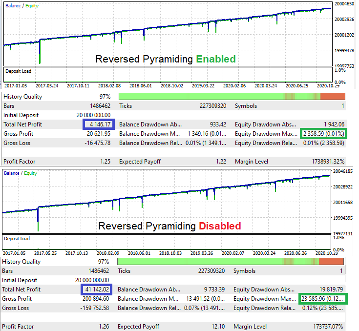
If you calculate D for the original test, it will take the value of 1.744. With the new mode enabled, this value is 1.758. Profitability has slightly shifted in the right direction. Of course, if we perform a few more tests, this value may fall, but on average there should be an increase in the variable. Strictly speaking, the logic is enough for demonstration.

Conclusion

In this article, I tried to collect the most interesting and useful techniques that can be helpful for automated trading system developers. Some of these techniques can assist in improving profits, after proper study and research. I hope this material is interesting and helpful. These techniques can be considered as a toolbox, but not a guide on how to build a Grail. Even a simple acquaintance with such techniques can save you from rash investments or critical losses. By investing more time and effort, you can try to create something more interesting and stable, than a conventional trading system based on the intersection of two indicators.