
Using Self-Organizing Feature Maps (Kohonen Maps) in MetaTrader 5

Introduction
A Self-Organizing Feature Map (SOM) is a type of artificial neural network that is trained using unsupervised learning to produce a two-dimensional discretized representation of the input space of the training samples, called a map.
These maps are useful for classification and visualizing low-dimensional views of high-dimensional data, akin to multidimensional scaling. The model was first described as an artificial neural network by the Finnish professor Teuvo Kohonen, and is sometimes called a Kohonen Map.
There are many algorithms available, we will follow the code, presented at http://www.ai-junkie.com. To visualize the data in MetaTrader 5 client terminal we will use the cIntBMP - a library for creation of BMP images. In this article we will consider several simple applications of Kohonen Maps.
1. Self-Organizing Feature Maps
The Self-Organizing Feature Maps were first described by Teuvo Kohonen in 1982. In contrast to many neural networks, it doesn't need one-to-one correspondence between the input and target output data. This neural network is trained using unsupervised learning.
The SOM may be described formally as a nonlinear, ordered, smooth mapping of high-dimensional input data onto the elements of a regular, low-dimensional array. In its basic form it produces a similarity graph of input data.
The SOM converts the nonlinear statistical relationships between high-dimensional data into simple geometric relationship of their image points on a regular two-dimensional grid of nodes. The SOM maps can be used for classification and visualizing of high-dimensional data.
1.1. Network Architecture
The simple Kohonen map as grid of 16 nodes (4x4 each of them is connected with 3-dimensional input vector) is presented in Fig. 1.
")
Figure 1. Simple Kohonen map (16 nodes)
Each node has (x,y) coordinates in lattice and vector of weights with components, defined in basis of the input vector.
1.2. Learning Algorithm
Unlike many other types of neural nets, the SOM doesn't need a target output to be specified. Instead, where the node weights match the input vector, that area of the lattice is selectively optimized to more closely resemble the data for the class the input vector is a member of.
From an initial distribution of random weights, and over many iterations, the SOM eventually settles into a map of stable zones. Each zone is effectively a feature classifier, so you can think of the graphical output as a type of feature map of the input space.
Training occurs in several steps and over many iterations:
- Each node's weights are initialized with random values.
- A vector is chosen randomly from the set of training data.
- Every node is examined to calculate which one's weights are most like the input vector. The winning node is commonly known as the Best Matching Unit (BMU).
- The radius of the neighbourhood of the BMU is calculated. Initially, this value is set to the radius of the lattice, but dimishless each time step.
- For any nodes found inside the radius of BMU, the node's weights are adjusted to make them more like the input vector. The closer a node to the BMU, the more its weights get alerted.
- Repeat step 2 for N iterations.
The details can be found at http://www.ai-junkie.com.
2. Case studies
2.1. Example 1. "Hello World!" in SOM
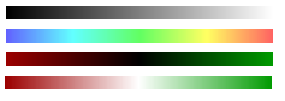
The classic example of Kohonen map is a color clustering problem.
Suppose we have a set of 8 colors, each of them is represented as a three dimensional vector in RGB color model.
-
 Red: (255,0,0);
  Green: (0,128,0);
 Blue: (0,0,255);
 Dark Green: (0,100,0);
 Dark Blue: (0,0,139);
 Yellow: (255,255,0);
 Orange: (255,165,0);
 Purple: (128,0,128).
When working with Kohonen maps in MQL5 language, we will follow the object-oriented paradigm.
We need two classes: CSOMNode class for a node of the regular grid and CSOM which is a neural network class.
//+------------------------------------------------------------------+
//| CSOMNode class                                                   |
//+------------------------------------------------------------------+
class CSOMNode
  {
protected:
   int               m_x1;
   int               m_y1;
   int               m_x2;
   int               m_y2;

   double            m_x;
   double            m_y;
   double            m_weights[];
public:
   //--- class constructor
                     CSOMNode();
   //--- class destructor
                    ~CSOMNode();
   //--- node initialization
   void              InitNode(int x1,int y1,int x2,int y2);
   //--- return coordinates of the node's center
   double            X()  const { return(m_x);}
   double            Y()  const { return(m_y);}
   //--- returns the node coordinates
   void              GetCoordinates(int &x1,int &y1,int &x2,int &y2);
   //--- returns the value of weight_index component of weight's vector
   double            GetWeight(int weight_index);
   //--- returns the squared distance between the node weights and specified vector
   double            CalculateDistance(double &vector[]);
   //--- adjust weights of the node
   void              AdjustWeights(double &vector[],double learning_rate,double influence);
  };
The implementation of class methods can be found in som_ex1.mq5. The code has a lot comments, we will focus on the idea.
The CSOM class description looks as follows:
//+------------------------------------------------------------------+
//| CSOM class                                                       |
//+------------------------------------------------------------------+
class CSOM
  {
protected:
   //--- class for using of bmp images
   cIntBMP           m_bmp;
   //--- grid mode
   int               m_gridmode;
   //--- bmp image size
   int               m_xsize;
   int               m_ysize;
   //--- number of nodes
   int               m_xcells;
   int               m_ycells;
   //--- array with nodes
   CSOMNode          m_som_nodes[];
   //--- total items in training set
   int               m_total_training_sets;
   //--- training set array
   double            m_training_sets_array[];
protected:
   //--- radius of the neighbourhood (used for training)
   double            m_map_radius;
   //--- time constant (used for training)
   double            m_time_constant;
   //--- initial learning rate (used for training)
   double            m_initial_learning_rate;
   //--- iterations (used for training)
   int               m_iterations;

public:
   //--- class constructor
                     CSOM();
   //--- class destructor
                    ~CSOM();
   //--- net initialization
   void              InitParameters(int iterations,int xcells,int ycells,int bmpwidth,int bmpheight);
   //--- finds the best matching node, closest to the specified vector
   int               BestMatchingNode(double &vector[]);
   //--- train method
   void              Train();
   //--- render method
   void              Render();
   //--- shows the bmp image on the chart
   void              ShowBMP(bool back);
   //--- adds a vector to training set
   void              AddVectorToTrainingSet(double &vector[]);
   //--- shows the pattern title
   void              ShowPattern(double c1,double c2,double c3,string name);
   //--- adds a pattern to training set
   void              AddTrainPattern(double c1,double c2,double c3);
   //--- returns the RGB components of the color
   void              ColToRGB(int col,int &r,int &g,int &b);
   //--- returns the color by RGB components
   int               RGB256(int r,int g,int b) const {return(r+256*g+65536*b);      }
   //--- deletes image from the chart
   void              NetDeinit();
  };
The use of the CSOM class is simple:
CSOM KohonenMap;
//+------------------------------------------------------------------+
//| Expert initialization function                                   |
//+------------------------------------------------------------------+
void OnInit()
  {
  MathSrand(200);
//--- initialize net, 10000 iterations will be used for training
//--- the net contains 15x20 nodes, bmp image size 400x400
   KohonenMap.InitParameters(10000,15,20,400,400);
//-- add RGB-components of each color from training set
   KohonenMap.AddTrainPattern(255,  0,  0);   // Red
   KohonenMap.AddTrainPattern(  0,128,  0);   // Green
   KohonenMap.AddTrainPattern(  0,  0,255);   // Blue
   KohonenMap.AddTrainPattern(  0,100,  0);   // Dark green
   KohonenMap.AddTrainPattern(  0,  0,139);   // Dark blue
   KohonenMap.AddTrainPattern(255,255,  0);   // Yellow
   KohonenMap.AddTrainPattern(255,165,  0);   // Orange
   KohonenMap.AddTrainPattern(128,  0,128);   // Purple
//--- train net
   KohonenMap.Train();
//--- render map to bmp
   KohonenMap.Render();
//--- show patterns and titles for each color
   KohonenMap.ShowPattern(255,  0,  0,"Red");
   KohonenMap.ShowPattern(  0,128,  0,"Green");
   KohonenMap.ShowPattern(  0,  0,255,"Blue");
   KohonenMap.ShowPattern(  0,100,  0,"Dark green");
   KohonenMap.ShowPattern(  0,  0,139,"Dark blue");
   KohonenMap.ShowPattern(255,255,  0,"Yellow");
   KohonenMap.ShowPattern(255,165,  0,"Orange");
   KohonenMap.ShowPattern(128,  0,128,"Purple");
//--- show bmp image on the chart
   KohonenMap.ShowBMP(false);
//---
  }
The result is presented in Fig. 2.

Figure 2. The output of SOM_ex1.mq5 Expert Advisor
The dynamics of Kohonen map learning is presented in Fig. 3 (see steps below the image):

Figure 3. The dynamics of Kohonen Map learning
One can see from the Fig. 3, the Kohonen Map is formed after 2400 steps.
If we create the lattice of 300 nodes and specify the image size as 400x400:
//--- lattice of 15x20 nodes, image size 400x400
   KohonenMap.InitParameters(10000,15,20,400,400);
we will get the image, presented in Fig. 4:

Figure 4. The Kohonen Map with 300 nodes, image size 400x400
If you read the Visual Explorations in Finance: with Self-Organizing Maps book, written by Guido Deboeck and Teuvo Kohonen, you remember that lattice nodes also can be represented as hexagonal cells. By modifying the code of the Expert Advisor, we can implement another visualization.
The result of SOM-ex1-hex.mq5 is presented in Fig. 5:

Figure 5. The Kohonen Map with 300 nodes, image size 400x400, the nodes are represented at hexagonal cells
In this version we can define the showing of cell borders by using the input parameters:
// input parameter, used to show hexagonal cells
input bool HexagonalCell=true;
// input parameter, used to show borders
input bool ShowBorders=true;
In some case we don't need to show the cell borders, if you specify ShowBorders=false, you will get the following image (see Fig. 6):

Fig. 6. Kohonen Map with 300 nodes, image 400x400, nodes plotted as hexagonal cells, cell borders disabled
In first example we have used 8 colors in training set with specified the color components. We can extend the training set and simplify the specifying of color components by adding two methods to CSOM class.
Note that in this case Kohonen Maps are simple because there are just few colors, separated in the color space. As a result, we have got the localized clusters.
The problem appears if we consider more colors with closer color components.
2.2. Example 2. Using Web-colors as training samples
In MQL5 Language the Web-colors are predefined constants.

Figure 7. Web-colors
What if we apply the Kohonen algorithm to a set of vectors with similar components?
We can create a CSOMWeb class, derived from CSOM class:
//+------------------------------------------------------------------+
//| CSOMWeb class                                                    |
//+------------------------------------------------------------------+
class CSOMWeb : public CSOM
  {
public:
//--- adds a color to training set (used for colors, instead of AddTrainPattern)
   void              AddTrainColor(int col);
//--- method of showing of title of the pattern (used for colors, instead of ShowPattern)
   void              ShowColor(int col,string name);
  };
As you see, to simplify the work with colors, we have added two new methods, the explicit specifying of color components isn't needed now.
The implementation of class methods looks as follows:
//+------------------------------------------------------------------+
//| Adds a color to training set                                     |
//| (used for colors, instead of AddTrainPattern)                    |
//+------------------------------------------------------------------+
void CSOMWeb::AddTrainColor(int col)
  {
   double vector[];
   ArrayResize(vector,3);
   int r=0;
   int g=0;
   int b=0;
   ColToRGB(col,r,g,b);
   vector[0]=r;
   vector[1]=g;
   vector[2]=b;
   AddVectorToTrainingSet(vector);
   ArrayResize(vector,0);
  }
//+------------------------------------------------------------------+
//| Method of showing of title of the pattern                        |
//| (used for colors, instead of ShowPattern)                        |
//+------------------------------------------------------------------+
void CSOMWeb::ShowColor(int col,string name)
  {
   int r=0;
   int g=0;
   int b=0;
   ColToRGB(col,r,g,b);
   ShowPattern(r,g,b,name);
  }
All web color can be combined in web_colors[] array:
//--- web colors array
color web_colors[132]=
  {
   clrBlack, clrDarkGreen, clrDarkSlateGray, clrOlive, clrGreen,
   clrTeal, clrNavy, clrPurple, clrMaroon, clrIndigo, clrMidnightBlue,
   clrDarkBlue, clrDarkOliveGreen, clrSaddleBrown, clrForestGreen, clrOliveDrab,
   clrSeaGreen, clrDarkGoldenrod, clrDarkSlateBlue, clrSienna, clrMediumBlue,
   clrBrown, clrDarkTurquoise, clrDimGray, clrLightSeaGreen, clrDarkViolet,
   clrFireBrick, clrMediumVioletRed, clrMediumSeaGreen, clrChocolate, clrCrimson,
   clrSteelBlue, clrGoldenrod, clrMediumSpringGreen, clrLawnGreen, clrCadetBlue,
   clrDarkOrchid, clrYellowGreen, clrLimeGreen, clrOrangeRed, clrDarkOrange,
   clrOrange, clrGold, clrYellow, clrChartreuse, clrLime, clrSpringGreen,
   clrAqua, clrDeepSkyBlue, clrBlue, clrMagenta, clrRed, clrGray,
   clrSlateGray, clrPeru, clrBlueViolet, clrLightSlateGray, clrDeepPink,
   clrMediumTurquoise, clrDodgerBlue, clrTurquoise, clrRoyalBlue, clrSlateBlue,
   clrDarkKhaki, clrIndianRed, clrMediumOrchid, clrGreenYellow, clrMediumAquamarine,
   clrDarkSeaGreen, clrTomato, clrRosyBrown, clrOrchid, clrMediumPurple,
   clrPaleVioletRed, clrCoral, clrCornflowerBlue, clrDarkGray, clrSandyBrown,
   clrMediumSlateBlue, clrTan, clrDarkSalmon, clrBurlyWood, clrHotPink,
   clrSalmon, clrViolet, clrLightCoral, clrSkyBlue, clrLightSalmon,
   clrPlum, clrKhaki, clrLightGreen, clrAquamarine, clrSilver,
   clrLightSkyBlue, clrLightSteelBlue, clrLightBlue, clrPaleGreen, clrThistle,
   clrPowderBlue, clrPaleGoldenrod, clrPaleTurquoise, clrLightGray, clrWheat,
   clrNavajoWhite, clrMoccasin, clrLightPink, clrGainsboro, clrPeachPuff,
   clrPink, clrBisque, clrLightGoldenrod, clrBlanchedAlmond, clrLemonChiffon,
   clrBeige, clrAntiqueWhite, clrPapayaWhip, clrCornsilk, clrLightYellow,
   clrLightCyan, clrLinen, clrLavender, clrMistyRose, clrOldLace,
   clrWhiteSmoke, clrSeashell, clrIvory, clrHoneydew, clrAliceBlue,
   clrLavenderBlush, clrMintCream, clrSnow, clrWhite
  };
The OnInit() function has simple form:
CSOMWeb KohonenMap;
//+------------------------------------------------------------------+
//| Expert initialization function                                   |
//+------------------------------------------------------------------+
void OnInit()
  {
   MathSrand(200);
   int total_web_colors=ArraySize(web_colors);
//--- initialize net, 10000 iterations will be used for training
//--- the net contains 15x20 nodes, bmp image size 400x400
   KohonenMap.InitParameters(10000,50,50,500,500);
//-- add all web colors to training set
   for(int i=0; i<total_web_colors; i++)
     {
      KohonenMap.AddTrainColor(web_colors[i]);
     }
//--- train net
   KohonenMap.Train();
//--- render map to bmp
   KohonenMap.Render();
//--- show patterns and titles for each color
   for(int i=0; i<total_web_colors; i++)
     {
      KohonenMap.ShowColor(web_colors[i],ColorToString(web_colors[i],true));
     }
//--- show bmp image on the chart
   KohonenMap.ShowBMP(false);
  }
If we launch the som-ex2-hex.mq5, we will get the picture, presented in Fig. 8.

Figure 8. Kohonen Map for Web-colors
As you see, there are some clusters, but some colors (like xxxBlue) are located in different regions.
The reason of this fact is the structure of training set, there are many vectors with close components.
2.3. Example 3. Product clustering
Next we will consider a simple example that will attempt to group twenty-five foods into regions of similarity, based on three parameters, which are protein, carbohydrate and fat.
| Food | Protein | Carbohydrate | Fat | |
|---|---|---|---|---|
| 1 | Apples | 0.4 | 11.8 | 0.1 |
| 2 | Avocado | 1.9 | 1.9 | 19.5 |
| 3 | Bananas | 1.2 | 23.2 | 0.3 |
| 4 | Beef Steak | 20.9 | 0 | 7.9 |
| 5 | Big Mac | 13 | 19 | 11 |
| 6 | Brazil Nuts | 15.5 | 2.9 | 68.3 |
| 7 | Bread | 10.5 | 37 | 3.2 |
| 8 | Butter | 1 | 0 | 81 |
| 9 | Cheese | 25 | 0.1 | 34.4 |
| 10 | Cheesecake | 6.4 | 28.2 | 22.7 |
| 11 | Cookies | 5.7 | 58.7 | 29.3 |
| 12 | Cornflakes | 7 | 84 | 0.9 |
| 13 | Eggs | 12.5 | 0 | 10.8 |
| 14 | Fried Chicken | 17 | 7 | 20 |
| 15 | Fries | 3 | 36 | 13 |
| 16 | Hot Chocolate | 3.8 | 19.4 | 10.2 |
| 17 | Pepperoni | 20.9 | 5.1 | 38.3 |
| 18 | Pizza | 12.5 | 30 | 11 |
| 19 | Pork Pie | 10.1 | 27.3 | 24.2 |
| 20 | Ptatoes | 1.7 | 16.1 | 0.3 |
| 21 | Rice | 6.9 | 74 | 2.8 |
| 22 | Roast Chicken | 26.1 | 0.3 | 5.8 |
| 23 | Sugar | 0 | 95.1 | 0 |
| 24 | Tuna Steak | 25.6 | 0 | 0.5 |
| 25 | Water | 0 | 0 | 0 |
Table 1. Protein, carbohydrate and fat for 25 foods.
This problem is interesting, because input vectors have different values and each components has its own range of values. It's important for visualization, because we use the RGB color model with components vary from 0 to 255.
Fortunately, in this case the input vectors are also 3-dimensional and we can use the RGB color model for Kohonen map visualization.
//+------------------------------------------------------------------+
//| CSOMFood class                                                   |
//+------------------------------------------------------------------+
class CSOMFood : public CSOM
  {
protected:
   double            m_max_values[];
   double            m_min_values[];
public:
   void              Train();
   void              Render();
   void              ShowPattern(double c1,double c2,double c3,string name);
  };
As you see, we have added m_max_values[] and m_min_values[] arrays for storage of maximal and minimal values of training set. For visualization in RGB-color model, the "scaling" is needed, so we have overloaded the Train(), Render() and ShowPattern() methods.
The search of the maximal and minimal values is implemented in Train() method.
//--- find minimal and maximal values of the training set
   ArrayResize(m_max_values,3);
   ArrayResize(m_min_values,3);

   for(int j=0; j<3; j++)
     {
      double maxv=m_training_sets_array[3+j];
      double minv=m_training_sets_array[3+j];
      for(int i=1; i<m_total_training_sets; i++)
        {
         double v=m_training_sets_array[3*i+j];
         if(v>maxv) {maxv=v;}
         if(v<minv) {minv=v;}
        }
      m_max_values[j]=maxv;
      m_min_values[j]=minv;
      Print(j,"m_min_value=",m_min_values[j],"m_max_value=",m_max_values[j]);
     }
To show the components in RGB color model, we need to modify the Render() method:
// int r = int(m_som_nodes[ind].GetWeight(0));
// int g = int(m_som_nodes[ind].GetWeight(1));
// int b = int(m_som_nodes[ind].GetWeight(2));

int r=int ((255*(m_som_nodes[ind].GetWeight(0)-m_min_values[0])/(m_max_values[0]-m_min_values[0])));
int g=int ((255*(m_som_nodes[ind].GetWeight(1)-m_min_values[1])/(m_max_values[1]-m_min_values[1])));
int b=int ((255*(m_som_nodes[ind].GetWeight(2)-m_min_values[2])/(m_max_values[2]-m_min_values[2])));
The result of som_ex3.mq5 is presented in Fig. 9.

Figure 9. Food map, grouped into regions of similarity, based on protein, carbohydrate and fat
Component analysis. One can see from the map, that Sugar, Rice and Cornflakes are plotted with green color because of the Carbohydrate (2nd component). The Butter is in green zone, it has a lot of Fat (3rd component). A lot of Protein (1st component, red) is contained in Beef Steak, Roast Chicken and Tuna Steak.
You can extend the training set by adding new food from the Food Composition Tables (alternative table).
As you see, the problem is solved for "pure" R,G,B directions. What about other foods with several equal (or mostly equal) components? Futher we will consider the Component Planes, it's very useful, especially for cases when input vectors have dimension, greater than 3.
2.4. Example 4. 4-dimensional case. Fisher's Iris data set. CMYK
For three-dimensional vectors, there is no problem with visualization. The results are clear because of RGB-color model, used to visualize color components.
When working with high-dimensional data, we need to find the way to visualize them. The simple solution is to plot a gradient map (for example, Black/White), with colors, proportional to the vector length. The other way is to use another color spaces. In this example we will consider the CMYK color model for Fisher's Iris data set. There is a better solution, futher we will consider it.
The Iris flower data set or Fisher's Iris data set is a multivariate data set introduced by R. Fisher (1936) as an example of discriminant analysis. The dataset consists of 50 samples from each of three species of Iris flowers (Iris setosa, Iris virginica and Iris versicolor).
Four features were measured from each sample, they are the length and the width of sepal and petal, in centimeters.

Figure 10. Iris flower
Each sample has 4 characteristics:
- Sepal length;
- Sepal width;
- Petal length;
- Petal width.
The Iris flower data set can be found in SOM_ex4.mq5.
In this example we will use the intermediate CMYK-color space for plotting, i.e. we will consider the weights of the node as a vectors in CMYK space. To visualize the results, the CMYK->RGB conversion is used. A new method int CSOM::CMYK2Col(uchar c,uchar m,uchar y,uchar k) is added to CSOM class, it used in CSOM::Render() method. Also we have to modify the classes to support 4-dimensional vectors.
The result is presented in Fig. 11.

Figure 11. Kohonen Map for Iris flower data set, plotted in CMYK color model
What do we see? We haven't got the complete clustering (because of the problem's features), but one can see the linear separation of iris setosa.
The reason of this linear separation of setosa is a large "Magenta" component (2nd) in CMYK space.
2.6. Component Plane Analysis
One can see from the previous examples (food and iris data clustering) there is a problem with data visualization.
For example, for food problem, we analyzed the Kohonen Map using the information on certain colors (red, green, blue). In addition to basic clusters, there were some foods with several components. Moreover, the analysis became difficult if the components are mostly equal.
The component planes provide the possibility to see the relative intensity for each of the food.
We need to add the CIntBMP class instances (m_bmp[] array) into the CSOM class and modify the corresponding render methods. Also we need a gradient map to visualize the intensity of each component (the lower values shown with blue color, the higher values shown with red):
![]()
Figure 12. Gradient palette
We added the Palette[768] array, the GetPalColor() and Blend() methods. The drawing of a node is placed to RenderCell() method.
Iris Flower Data Set
The results of som-ex4-cpr.mq5 is presented in Fig. 13.

Figure 13. Component planes representation of the Iris flower data set
In this case we use the grid with 30x30 nodes, image size 300x300.
The component planes plays an important role in correlation detection: by comparing these planes even partiallly correlating variables may be detected by visual inspection. This is easier if the component planes are reorganized so that the correlated ones are near each other. In this way, it's easy to select interesting component combinations for further investigation.
Let's consider the component planes (Fig. 14).
The values of maximal and minimal components are shown in the gradient table.

Figure 14. Iris flower data set. Component planes
All these component planes, represented in the CMYK-color model are shown in Fig. 15.

Figure 15. Iris flower data set. Kohonen map in CMYK color model
Let's remind the setosa iris type. Using the component plane analysis (Fig. 14) one can see that it has minimal values in 1st (Sepal Length), 3rd (Petal Length) and 4th (Petal Width) component planes.
It's remarkable that it has maximal values in the 2nd component plane (Sepal Width), the same result we have got in CMYK-color model (Magenta component, Fig. 15).
Food Clustering
Now let's consider food clustering problem using the component plane analysis (som-ex3-cpr.mq5).
The result is presented in Fig. 16 (30x30 nodes, image size 300x300, hexagonal cells without borders).

Figure 16. Kohonen map for food, component plane representation
We added the showing of titles option in ShowPattern() method of CSOM class (input parameter ShowTitles=true).
The component planes (protein, carbohydrate, fat) looks as follows:

Figure 17. Kohonen map for foods. Component planes and RGB color model
The component plane representation, shown in Fig. 17 opens a new view on the structure of food components. Moreover, it provides additional information, that cannot be seen in RGB color model, presented in Fig. 9.
For example, now we see the Cheese in the 1st component plane (protein). In RGB color model it shown with color, close to magenta, because of the fat (2nd component).
2.5. Implementation of Component Planes for the Case of Arbitrary Dimension
The examples we have considered have some specific features, the dimension was fixed and visualization algorithm was different for different representations (RGB and CMYK color models).
Now we can generalize the algorithm for arbitrary dimensions, but in this case we will visualize the component planes only. The program must be able to load the arbitrary data from CSV file.
For example, the food.csv looks as follows:
Protein;Carbohydrate;Fat;Title
0.4;11.8;0.1;Apples
1.9;1.9;19.5;Avocado
1.2;23.2;0.3;Bananas
20.9;0.0;7.9;Beef Steak
13.0;19.0;11.0;Big Mac
15.5;2.9;68.3;Brazil Nuts
10.5;37.0;3.2;Bread
1.0;0.0;81.0;Butter
25.0;0.1;34.4;Cheese
6.4;28.2;22.7;Cheesecake
5.7;58.7;29.3;Cookies
7.0;84.0;0.9;Cornflakes
12.5;0.0;10.8;Eggs
17.0;7.0;20.0;Fried Chicken
3.0;36.0;13.0;Fries
3.8;19.4;10.2;Hot Chocolate
20.9;5.1;38.3;Pepperoni
12.5;30.0;11.0;Pizza
10.1;27.3;24.2;Pork Pie
1.7;16.1;0.3;Potatoes
6.9;74.0;2.8;Rice
26.1;0.3;5.8;Roast Chicken
0.0;95.1;0.0;Sugar
25.6;0.0;0.5;Tuna Steak
0.0;0.0;0.0;Water
The first line of the file contrain the names (titles) of the input data vector. The titles are needed to distingush the component planes, we will print their names in the gradient panel.
The name of the pattern is located in the last column, in our case it's the name of the food.
The code of SOM.mq5 (OnInit function) is simplified:
CSOM KohonenMap;
//+------------------------------------------------------------------+
//| Expert initialization function                                   |
//+------------------------------------------------------------------+
int OnInit()
  {
   MathSrand(200);
//--- load patterns from file
   if(!KohonenMap.LoadTrainDataFromFile(DataFileName))
     {
      Print("Error in loading data for training.");
      return(1);
     }
//--- train net
   KohonenMap.Train();
//--- render map
   KohonenMap.Render();
//--- show patterns from training set
   KohonenMap.ShowTrainPatterns();
//--- show bmp on the chart
   KohonenMap.ShowBMP(false);
   return(0);
  }
The name of the file with training patterns is specified in DataFileName input parameter, in our case "food.csv".
The result is shown in Fig. 18.

Figure 18. Kohonen Map of food in black/white gradient color scheme
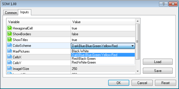
Also we added the ColorScheme input parameter for gradient scheme selection.
At present time there are 4 color schemes available (ColorScheme=0,1,2,4=Black-White, DarkBlue-Blue-Green-Yellow-Red, Red-Black-Green, Red-White-Green).
You can easy add your own scheme by adding the gradient into the CSOM::InitParameters() method.
The color scheme can be selected from the input parameters of Expert Advisor:
Similarly we can prepare the Iris flower data set (iris-fisher.csv):
Sepal length;Sepal width;Petal length;Petal width;Title
5.1;3.5;1.4;0.2;setosa
4.9;3.0;1.4;0.2;setosa
4.7;3.2;1.3;0.2;setosa
4.6;3.1;1.5;0.2;setosa
5.0;3.6;1.4;0.2;setosa
5.4;3.9;1.7;0.4;setosa
4.6;3.4;1.4;0.3;setosa
5.0;3.4;1.5;0.2;setosa
4.4;2.9;1.4;0.2;setosa
4.9;3.1;1.5;0.1;setosa
5.4;3.7;1.5;0.2;setosa
4.8;3.4;1.6;0.2;setosa
4.8;3.0;1.4;0.1;setosa
4.3;3.0;1.1;0.1;setosa
5.8;4.0;1.2;0.2;setosa
5.7;4.4;1.5;0.4;setosa
5.4;3.9;1.3;0.4;setosa
5.1;3.5;1.4;0.3;setosa
5.7;3.8;1.7;0.3;setosa
5.1;3.8;1.5;0.3;setosa
5.4;3.4;1.7;0.2;setosa
5.1;3.7;1.5;0.4;setosa
4.6;3.6;1.0;0.2;setosa
5.1;3.3;1.7;0.5;setosa
4.8;3.4;1.9;0.2;setosa
5.0;3.0;1.6;0.2;setosa
5.0;3.4;1.6;0.4;setosa
5.2;3.5;1.5;0.2;setosa
5.2;3.4;1.4;0.2;setosa
4.7;3.2;1.6;0.2;setosa
4.8;3.1;1.6;0.2;setosa
5.4;3.4;1.5;0.4;setosa
5.2;4.1;1.5;0.1;setosa
5.5;4.2;1.4;0.2;setosa
4.9;3.1;1.5;0.2;setosa
5.0;3.2;1.2;0.2;setosa
5.5;3.5;1.3;0.2;setosa
4.9;3.6;1.4;0.1;setosa
4.4;3.0;1.3;0.2;setosa
5.1;3.4;1.5;0.2;setosa
5.0;3.5;1.3;0.3;setosa
4.5;2.3;1.3;0.3;setosa
4.4;3.2;1.3;0.2;setosa
5.0;3.5;1.6;0.6;setosa
5.1;3.8;1.9;0.4;setosa
4.8;3.0;1.4;0.3;setosa
5.1;3.8;1.6;0.2;setosa
4.6;3.2;1.4;0.2;setosa
5.3;3.7;1.5;0.2;setosa
5.0;3.3;1.4;0.2;setosa
7.0;3.2;4.7;1.4;versicolor
6.4;3.2;4.5;1.5;versicolor
6.9;3.1;4.9;1.5;versicolor
5.5;2.3;4.0;1.3;versicolor
6.5;2.8;4.6;1.5;versicolor
5.7;2.8;4.5;1.3;versicolor
6.3;3.3;4.7;1.6;versicolor
4.9;2.4;3.3;1.0;versicolor
6.6;2.9;4.6;1.3;versicolor
5.2;2.7;3.9;1.4;versicolor
5.0;2.0;3.5;1.0;versicolor
5.9;3.0;4.2;1.5;versicolor
6.0;2.2;4.0;1.0;versicolor
6.1;2.9;4.7;1.4;versicolor
5.6;2.9;3.6;1.3;versicolor
6.7;3.1;4.4;1.4;versicolor
5.6;3.0;4.5;1.5;versicolor
5.8;2.7;4.1;1.0;versicolor
6.2;2.2;4.5;1.5;versicolor
5.6;2.5;3.9;1.1;versicolor
5.9;3.2;4.8;1.8;versicolor
6.1;2.8;4.0;1.3;versicolor
6.3;2.5;4.9;1.5;versicolor
6.1;2.8;4.7;1.2;versicolor
6.4;2.9;4.3;1.3;versicolor
6.6;3.0;4.4;1.4;versicolor
6.8;2.8;4.8;1.4;versicolor
6.7;3.0;5.0;1.7;versicolor
6.0;2.9;4.5;1.5;versicolor
5.7;2.6;3.5;1.0;versicolor
5.5;2.4;3.8;1.1;versicolor
5.5;2.4;3.7;1.0;versicolor
5.8;2.7;3.9;1.2;versicolor
6.0;2.7;5.1;1.6;versicolor
5.4;3.0;4.5;1.5;versicolor
6.0;3.4;4.5;1.6;versicolor
6.7;3.1;4.7;1.5;versicolor
6.3;2.3;4.4;1.3;versicolor
5.6;3.0;4.1;1.3;versicolor
5.5;2.5;4.0;1.3;versicolor
5.5;2.6;4.4;1.2;versicolor
6.1;3.0;4.6;1.4;versicolor
5.8;2.6;4.0;1.2;versicolor
5.0;2.3;3.3;1.0;versicolor
5.6;2.7;4.2;1.3;versicolor
5.7;3.0;4.2;1.2;versicolor
5.7;2.9;4.2;1.3;versicolor
6.2;2.9;4.3;1.3;versicolor
5.1;2.5;3.0;1.1;versicolor
5.7;2.8;4.1;1.3;versicolor
6.3;3.3;6.0;2.5;virginica
5.8;2.7;5.1;1.9;virginica
7.1;3.0;5.9;2.1;virginica
6.3;2.9;5.6;1.8;virginica
6.5;3.0;5.8;2.2;virginica
7.6;3.0;6.6;2.1;virginica
4.9;2.5;4.5;1.7;virginica
7.3;2.9;6.3;1.8;virginica
6.7;2.5;5.8;1.8;virginica
7.2;3.6;6.1;2.5;virginica
6.5;3.2;5.1;2.0;virginica
6.4;2.7;5.3;1.9;virginica
6.8;3.0;5.5;2.1;virginica
5.7;2.5;5.0;2.0;virginica
5.8;2.8;5.1;2.4;virginica
6.4;3.2;5.3;2.3;virginica
6.5;3.0;5.5;1.8;virginica
7.7;3.8;6.7;2.2;virginica
7.7;2.6;6.9;2.3;virginica
6.0;2.2;5.0;1.5;virginica
6.9;3.2;5.7;2.3;virginica
5.6;2.8;4.9;2.0;virginica
7.7;2.8;6.7;2.0;virginica
6.3;2.7;4.9;1.8;virginica
6.7;3.3;5.7;2.1;virginica
7.2;3.2;6.0;1.8;virginica
6.2;2.8;4.8;1.8;virginica
6.1;3.0;4.9;1.8;virginica
6.4;2.8;5.6;2.1;virginica
7.2;3.0;5.8;1.6;virginica
7.4;2.8;6.1;1.9;virginica
7.9;3.8;6.4;2.0;virginica
6.4;2.8;5.6;2.2;virginica
6.3;2.8;5.1;1.5;virginica
6.1;2.6;5.6;1.4;virginica
7.7;3.0;6.1;2.3;virginica
6.3;3.4;5.6;2.4;virginica
6.4;3.1;5.5;1.8;virginica
6.0;3.0;4.8;1.8;virginica
6.9;3.1;5.4;2.1;virginica
6.7;3.1;5.6;2.4;virginica
6.9;3.1;5.1;2.3;virginica
5.8;2.7;5.1;1.9;virginica
6.8;3.2;5.9;2.3;virginica
6.7;3.3;5.7;2.5;virginica
6.7;3.0;5.2;2.3;virginica
6.3;2.5;5.0;1.9;virginica
6.5;3.0;5.2;2.0;virginica
6.2;3.4;5.4;2.3;virginica
5.9;3.0;5.1;1.8;virginica
The result is shown in Fig. 19.
")
Figure 19. Iris flower data set. Component planes in Red-Black-Green color scheme (ColorScheme=2, iris-fisher.csv)
Now we have a tool for the real applications.
2.6. Example 5. Market heat maps
Self-Organizing Feature Maps can be used for the market movement maps. Sometimes the global picture of the market is needed, the market heat map is a very useful tool. The stocks are combined together depending on economic sectors.
The current color of stock depends on current growth rate (in %):

Figure 20. Market heat map for stocks from S&P500
The weekly market heat map of the stocks from S&P (http://finviz.com) is shown in Fig. 20. The color depends on the growth rate (in %):
![]()
The size of the stock rectangle depends on market capitalization. The same analysis can be done in MetaTrader 5 client terminal using the Kohonen Maps.
The idea is to use the growth rates (in %) for several timeframes. We have the tool for working with Kohonen maps, so the only needed is the script, that saves the data to .csv file.
The price data on CFD prices of American stocks (#AA, #AIG, #AXP, #BA, #BAC, #C, #CAT, #CVX, #DD, #DIS, #EK, #GE, #HD, #HON, #HPQ, #IBM, #INTC, #IP, #JNJ, #JPM, #KFT, #KO, #MCD, #MMM, #MO, #MRK, #MSFT, #PFE, #PG, #T, #TRV, #UTX, #VZ, #WMT и #XOM) can be found at MetaQuotes Demo server.
The script, that prepares the dj.csv file is very simple:
//+------------------------------------------------------------------+
//|                                                           DJ.mq5 |
//|                        Copyright 2011, MetaQuotes Software Corp. |
//|                                              https://www.mql5.com |
//+------------------------------------------------------------------+
#property copyright "Copyright 2011, MetaQuotes Software Corp."
#property link      "https://www.mql5.com"
#property version   "1.00"

string s_cfd[35]=
  {
   "#AA","#AIG","#AXP","#BA","#BAC","#C","#CAT","#CVX","#DD","#DIS","#EK","#GE",
   "#HD","#HON","#HPQ","#IBM","#INTC","#IP","#JNJ","#JPM","#KFT","#KO","#MCD","#MMM",
   "#MO","#MRK","#MSFT","#PFE","#PG","#T","#TRV","#UTX","#VZ","#WMT","#XOM"
  };
//+------------------------------------------------------------------+
//| Returns price change in percents                                 |
//+------------------------------------------------------------------+
double PercentChange(double Open,double Close)
  {
   return(100.0*(Close-Open)/Close);
  }
//+------------------------------------------------------------------+
//| Script program start function                                    |
//+------------------------------------------------------------------+
void OnStart()
  {

   ResetLastError();
   int filehandle=FileOpen("dj.csv",FILE_WRITE|FILE_ANSI);
   if(filehandle==INVALID_HANDLE)
     {
      Alert("Error opening file");
      return;
     }
//---
   MqlRates MyRates[];
   ArraySetAsSeries(MyRates,true);

   string t="M30;M60;M90;M120;M150;M180;M210;M240;Title";
   FileWrite(filehandle,t);
   Print(t);

   int total_symbols=ArraySize(s_cfd);

   for(int i=0; i<total_symbols; i++)
     {
      string cursymbol=s_cfd[i];

      int copied1=CopyRates(cursymbol,PERIOD_M30,0,8,MyRates);
      if(copied1>0)
        {
         string s="";
         s=s+DoubleToString(PercentChange(MyRates[1].open,MyRates[0].close),3)+";";
         s=s+DoubleToString(PercentChange(MyRates[2].open,MyRates[0].close),3)+";";
         s=s+DoubleToString(PercentChange(MyRates[3].open,MyRates[0].close),3)+";";
         s=s+DoubleToString(PercentChange(MyRates[4].open,MyRates[0].close),3)+";";
         s=s+DoubleToString(PercentChange(MyRates[5].open,MyRates[0].close),3)+";";
         s=s+DoubleToString(PercentChange(MyRates[6].open,MyRates[0].close),3)+";";
         s=s+DoubleToString(PercentChange(MyRates[7].open,MyRates[0].close),3)+";";
         s=s+cursymbol;
         Print(s);
         FileWrite(filehandle,s);
         }
         else
           {
            Print("Error in request of historical data on symbol ",cursymbol);
            return;
           }
     }
   Alert("OK");
   FileClose(filehandle);

  }
//+------------------------------------------------------------------+
The historical data must be downloaded, you can do it automatically using the DownloadHistory script.
As a result of dj.mq5 script, we will get the dj.csv with the following data:
M30;M60;M90;M120;M150;M180;M210;M240;Title
0.063;-0.564;-0.188;0.376;0.251;0.313;0.627;0.439;#AA
-0.033;0.033;0.067;-0.033;0.067;-0.133;0.266;0.533;#AIG
-0.176;0.039;0.039;0.274;0.196;0.215;0.430;0.646;#AXP
-0.052;-0.328;-0.118;0.315;0.223;0.367;0.288;0.328;#BA
-0.263;-0.351;-0.263;0.000;-0.088;0.088;0.000;-0.088;#BAC
-0.224;-0.274;-0.374;-0.100;-0.274;-0.224;-0.324;-0.598;#C
-0.069;-0.550;-0.079;0.766;0.727;0.638;0.736;0.589;#CAT
-0.049;-0.168;0.099;0.247;0.187;0.049;0.355;0.266;#CVX
0.019;-0.058;0.058;0.446;0.174;0.349;0.136;-0.329;#DD
-0.073;-0.219;-0.146;0.267;0.170;0.292;0.170;0.267;#DIS
-1.099;-1.923;-1.099;0.275;0.275;0.275;-0.549;-1.374;#EK
-0.052;-0.310;-0.103;0.362;0.258;0.362;0.465;0.258;#GE
-0.081;-0.244;-0.326;-0.136;0.081;0.326;0.489;0.489;#HD
-0.137;-0.427;-0.171;0.427;0.445;0.342;0.325;0.359;#HON
-0.335;-0.363;-0.112;0.112;0.168;0.307;0.475;0.251;#HPQ
0.030;-0.095;0.065;0.190;0.071;0.214;0.279;0.327;#IBM
0.000;-0.131;-0.044;-0.088;-0.044;0.000;0.000;0.044;#INTC
-0.100;-0.200;-0.166;0.100;-0.067;0.033;-0.532;-0.798;#IP
-0.076;0.076;0.259;0.473;0.427;0.336;0.336;-0.076;#JNJ
-0.376;-0.353;-0.494;-0.259;-0.423;-0.329;-0.259;-0.541;#JPM
-0.057;-0.086;-0.029;0.086;0.114;0.057;0.257;-0.114;#KFT
0.059;-0.030;0.119;0.282;0.119;0.193;0.208;-0.119;#KO
-0.109;-0.182;0.206;0.352;0.279;0.473;0.521;0.194;#MCD
-0.043;-0.195;-0.151;0.216;0.270;0.227;0.411;0.206;#MMM
-0.036;-0.072;0.072;0.144;-0.072;-0.108;0.108;0.072;#MO
0.081;-0.081;0.027;0.081;-0.054;0.027;-0.027;-0.108;#MRK
0.083;0.083;0.041;0.331;0.083;0.248;0.166;0.041;#MSFT
0.049;0.000;0.243;0.680;0.194;0.243;0.340;0.097;#PFE
-0.045;0.060;0.104;0.015;-0.179;-0.149;-0.224;-0.224;#PG
0.097;-0.032;0.000;0.129;0.129;0.064;0.097;0.064;#T
-0.277;-0.440;-0.326;-0.358;-0.537;-0.619;-0.570;-0.733;#TRV
-0.081;-0.209;0.035;0.325;0.198;0.093;0.128;-0.035;#UTX
0.054;0.000;0.054;0.190;0.136;0.326;0.380;0.353;#VZ
-0.091;-0.091;-0.036;0.036;-0.072;0.000;0.145;-0.127;#WMT
-0.062;-0.211;0.087;0.198;0.186;0.050;0.347;0.508;#XOM
After launching the som.mq5(ColorScheme=3, CellsX=30,CellsY=30, ImageXSize=200, ImageXSize=200, DataFileName="dj.csv"), we will get 8 pictures, each of them corresponds to the time intervals of 30, 60, 90, 120, 150, 180, 210 and 240 minutes.
The Kohonen maps of the market growth rate data (American stocks) of 4 last hours of 23 may 2011 trade session are presented in Fig. 21.
.")
Figure 21. Kohonen maps for American stocks (last 4 hours of 23 may 2011 trade session).
One can see from the Fig. 21, the dynamics of #C (Citigroup Inc.), #T (AT&T Inc.), #JPM (JPMorgan Chase & Co), #BAC (Bank of America) is similar. They grouped in a long-term red cluster.
During last 1.5 hours (M30, M60, M90) its dynamics became green, but generally (M240) the stocks were in the red zone.
Using Kohonen maps, we can visualize the relative dynamics of stocks, find leaders and loosers and their enviroment. The elements with similar data forms clusters.
As we see from the Fig. 21a, the price of the Citigroup Inc stocks was the leader of falling. Generally, all the stocks of finance companies were in red zone.
")
Figure 21a. Market heat map on 23 may 2011 (Source: http://finviz.com)
Similarly, we can calculate the Kohonen maps of FOREX market (Fig. 22):
")
Figure 22. Kohonen map for FOREX market (24 may 2011, European session)
The following pairs are used: EURUSD, GBPUSD, USDCHF, USDJPY, USDCAD, AUDUSD, NZDUSD, USDSEK, AUDNZD, AUDCAD, AUDCHF, AUDJPY, CHFJPY, EURGBP, EURAUD, EURCHF, EURJPY, EURNZD, EURCAD, GBPCHF, GBPJPY, CADCHF.
The growth rates are exported to fx.csv using the fx.mq5 script.
M30;M60;M90;M120;M150;M180;M210;M240;Title
0.058;-0.145;0.045;-0.113;-0.038;-0.063;0.180;0.067;EURUSD
0.046;-0.100;0.078;0.094;0.167;0.048;0.123;0.160;GBPUSD
-0.048;0.109;-0.142;-0.097;-0.219;-0.143;-0.277;-0.236;USDCHF
0.042;0.097;0.043;-0.024;-0.009;-0.067;0.024;0.103;USDJPY
-0.045;0.162;0.155;0.239;0.217;0.246;0.157;0.227;USDCAD
0.095;-0.126;-0.018;-0.141;-0.113;-0.062;0.081;-0.005;AUDUSD
0.131;-0.028;0.167;0.096;-0.013;0.147;0.314;0.279;NZDUSD
-0.047;0.189;-0.016;0.107;0.084;0.076;-0.213;-0.133;USDSEK
-0.034;-0.067;-0.188;-0.227;-0.102;-0.225;-0.234;-0.291;AUDNZD
0.046;0.039;0.117;0.102;0.097;0.170;0.234;0.216;AUDCAD
0.057;-0.016;-0.158;-0.226;-0.328;-0.215;-0.180;-0.237;AUDCHF
0.134;-0.020;0.024;-0.139;-0.124;-0.127;0.107;0.098;AUDJPY
0.083;-0.009;0.184;0.084;0.208;0.082;0.311;0.340;CHFJPY
0.025;-0.036;-0.030;-0.200;-0.185;-0.072;0.058;-0.096;EURGBP
-0.036;-0.028;0.061;0.010;0.074;-0.006;0.088;0.070;EURAUD
0.008;-0.049;-0.098;-0.219;-0.259;-0.217;-0.094;-0.169;EURCHF
0.096;-0.043;0.085;-0.124;-0.049;-0.128;0.206;0.157;EURJPY
-0.073;-0.086;-0.119;-0.211;-0.016;-0.213;-0.128;-0.213;EURNZD
0.002;0.009;0.181;0.119;0.182;0.171;0.327;0.284;EURCAD
-0.008;0.004;-0.077;-0.015;-0.054;-0.127;-0.164;-0.080;GBPCHF
0.079;-0.005;0.115;0.079;0.148;-0.008;0.144;0.253;GBPJPY
0.013;-0.060;-0.294;-0.335;-0.432;-0.376;-0.356;-0.465;CADCHF
In addition to prices, you can use the values of the indicators at different timeframes.
2.6. Example 6. Analysis of Optimization Results
The Strategy Tester of MetaTrader 5 client terminal provides an opportunity to explore the structure of parameter space and find the best set of the strategy parameters. Also you can export the optimization results using the "Export to XML (MS Office Excel)" option from the context menu of "Optimization Results" tab.
The Tester Statistics is also included in the optimization results (41 columns):
- Result
- Profit
- Gross Profit
- Gross Loss
- Withdrawal
- Expected Payoff
- Profit Factor
- Recovery Factor
- Sharpe Ratio
- Margin Level
- Custom
- Minimal Balance
- Balance DD Maximal
- Balance DD Maximal (%)
- Balance DD Relative
- Balance DD Relative (%)
- Minimal Equity
- Equity DD Maximal
- Equity DD Maximal (%)
- Equity DD Relative
- Equity DD Relative (%)
- Trades
- Deals
- Short Trades
- Profit Short Trades
- Long Trades
- Profit Long Trades
- Profit Trades
- Loss Trades
- Max profit trade
- Max loss trade
- Max consecutive wins
- Max consecutive wins ($)
- Max consecutive profit
- Max consecutive profit count
- Max consecutive losses
- Max consecutive losses ($)
- Max consecutive loss
- Max consecutive loss count
- Avg consecutive wins
- Avg consecutive losses
The use of tester statistics allows to help in analysis of parameter space. It's remarkable that many parameters of the statistic are closely related and depends on trade performance results.
For example, the best trading results have the largest values of Profit, Profit Factor, Recovery Factor and Sharpe Ratio parameters. This fact allows to use them in analysis of the results.
Optimization Results of MovingAverage.mq5 Expert Advisor
In this chapter we will consider the analysis of the optimization results of MovingAverage.mq5 Expert Advisor, included in standard package of MetaTrader 5 client terminal. This Expert Advisor is based on crossover of price and moving average indicator. It has two input parameters: MovingPeriod and MovingShift, i.e. we will have the XML-file with 43 columns as a result.
We will not consider the 43-dimensional space of parameters, the most interesting are:
- Profit;
- Profit Factor;
- Recovery Factor;
- Sharpe Ratio;
- Trades;
- ProfitTrades(%);
- MovingPeriod;
- MovingShift;
Note, we have added the ProfitTrades (%) parameter (it's absent in the results), it means the percent of profitable deals and calculated as result of division of ProfitTrades (28) by Trades (22), multiplied by 100..
Let's prepare the optim.csv file with 9 columns for 400 sets of input parameters of MetaTrader 5 Strategy Tester.
Profit;Profit Factor;Recovery Factor;Sharpe Ratio;Trades;ProfitTrades(%);MovingPeriod;MovingShift;Title
-372.3;0.83;-0.51;-0.05;71;28.16901408;43;6;43
-345.79;0.84;-0.37;-0.05;66;27.27272727;50;6;50
...
Note, that we have used the value of MovingPeriod as a Title column, it will be used to "mark" the patterns on the Kohonen maps.
In Strategy Tester we have optimized the values of MovingPeriod and MovingShift with following parameters:
- Symbol - EURUSD,
- Period - H1,
- Tick generation mode - "1 Minute OHLC",
- Testing interval - 2011.01.01-2011.05.24,
- Optimization - Fast (genetic algorithm),
- Optimization - Balance max.
")
Figure 23. Kohonen map for optimization results of MovingAverage EA (component plane representation)
Let's consider the component planes of the upper row (Profit, Profit Factor, Recovery Factor и Sharpe Ratio).
They are combined in Fig. 24.

Figure 24. Component planes for Profit, Profit Factor, Recovery Factor and Sharpe Ratio parameters
The first, that we needed is to find the regions with the best optimization results.
One can see from the Fig. 24, the regions with maximal values are located in the upper left corner. The numbers correspond to the averaging period of Moving Average indicator (MovingPeriod parameter, we used it as a title). The numbers location is the same for all component planes. An each component plane has its own range of values, the values are printed in the gradient panel.
The best optimization results have the larges values of Profit, Profit Factor, Recovery Factor and Sharpe Ratio, so we have information about the regions on the map (outlined in Fig. 24).
The component planes for Trades, ProfitTrades(%), MovingPeriod and MovingShift are presented in Fig. 25.
, MovingPeriod and MovingShift parameters")
Figure 25. Component planes for Trades, ProfitTrades(%), MovingPeriod and MovingShift parameters
Component Plane Analysis
At first glance, there isn't any interesting information. The first 4 component planes (Profit, Profit Factor, Recovery Factor and Sharpe Ratio) looks similar, because they depends directly on performance of trade system.
One can see from the Fig. 24, the upper left region is very interesting (for example, best results may be achieved if we set the MovingPeriod from 45 to 50).
The Expert Advisor was tested at hourly timeframe of EURUSD, its strategy based on trend, we can consider these values as a "market trend" memory. If it's true, the market trend memory for the first half of 2011 is equal to 2 days.
Let's consider other component planes.

Figure 26. Component planes Trades-MovingPeriod
Looking in Fig. 26, we can see that lower values of MovingPeriod (blue regions) leads to the greater values of Trades (yellow-red regions). If the period of moving average is low, there are many crossovers (trades).
Also we can see this fact on the Trades component plane (green regions with numbers below 20).

Figure 27. Component planes Trades-MovingShift
The number of trades decreases (blue regions) with increasing MovingShift (ytellow-red regions). Comparing the component planes for MovingShift and Fig.24, one can see that MovingShift parameter isn't very important for performance of this trade strategy.
The percent of profitable trades ProfitTrades(%) doesn't depend directly on MovingPeriod or MovingShift, it's an integral characteristic of the trade system. In other words, the analysis of its correlation with input parameters has no meaning.
More complex trade strategies can be analyzed the similar way. You need to find the most important parameter(s) of your trade system and use it as a title.
Conclusion
The main advantage of Self-Organizing Feature Maps is the opportunity to produce a two-dimensional discretized representation of high-dimensional data. The data with similar characteristics form clusters, it simplifies the correlation analysis.
The details and other applications can be found in excellent book Visual Explorations in Finance: with Self-Organizing Maps by Guido Deboeck and Teuvo Kohonen.
Appendix
After the publication of the Russian version, Alex Sergeev has proposed the impoved version of classes(SOM_Alex-Sergeev_en.zip).
Changes list:
1. Showing of images has changed: cIntBMP::Show(int aX, int aY, string aBMPFileName, string aObjectName, bool aFromImages=true)
2. Added the feature to open folder with images:
#import "shell32.dll"
   int ShellExecuteW(int hwnd, string oper, string prog, string param, string dir, int show);
#import

input bool OpenAfterAnaliz=true; // open folder with maps after finish
Changes in CSOM class:
- Added a method CSOM::HideChart - hides chart.
- Added class members m_chart, m_wnd, m_x0, m_y0 - (chart, window, and coordinates to show images).
+ added m_sID - object names prefix. The prefix uses file name, by default "SOM" prefix is used. - All maps are saved to the folder with m_sID name.
- The bmp files are named by column name of the patterns.
- Modified the CSOM::ShowBMP method (maps saved in \Files folder insted of \Images, it works much faster).
- The CSOM::NetDeinit changed to CSOM::HideBMP.
- Modified the CSOM::ReadCSVData method, the first column contain titles.
- Added a flag to show intermediate maps in CSOM::Train(bool bShowProgress).
- The showing of intermediate maps in CSOM::Train is performed every 2 seconds (instead of iteration), the progress is shown on the chart using the Comment.
- Optimized names of some variables, class methods ordered by category.
The drawing of bmp is a very slow process. If you don't really need it, don't draw it every time.
The example of SOM images with optimization results are included in archive.
Translated from Russian by MetaQuotes Ltd.
Original article: https://www.mql5.com/ru/articles/283
Warning: All rights to these materials are reserved by MetaQuotes Ltd. Copying or reprinting of these materials in whole or in part is prohibited.
 Payments and payment methods
 Using WinInet in MQL5. Part 2: POST Requests and Files
 How to Add New UI Languages to the MetaTrader 5 Platform
 Decreasing Memory Consumption by Auxiliary Indicators
- Free trading apps
- Over 8,000 signals for copying
- Economic news for exploring financial markets
You agree to website policy and terms of use
I always look at the root, I knew no one would call it a neural network if Kohonen's maps couldn't predict.
they can't, training is there to deploy vectors of NS weights over training sets - the result is to cluster the data, but the response of the network itself is absent to other data - or rather it will be, but it will produce random values.
about the root... the name is not Kohonen's network, it's like Self Organising Maps (SOM).
UPD: I don't see the point in continuing the discussion, the second time the discussion is reduced to what is written in Wiki, and now to what a certain "Quoting S. Osovsky" wrote. I agree to remain in the captivity of my reasoning, which is not supported by the phrase "SOM Kohonen" can predict, and the reverse - they can not
they don't know how to do it, there is training to deploy vectors of NS weights over training sets - the result is to cluster the data, but the response of the network itself is absent on other data - or rather it will be, but it will produce random values.
about the root... the name is not Kohonen network, but Self Organising Maps (SOM).
UPD: I don't see the point in continuing the discussion, the second time the discussion is reduced to what is written in Wiki, and now to what is written by someone "Quoting S. Osovsky". I agree to remain in the captivity of my reasoning, which is not supported by the phrase "SOM Kohonen" can predict, and the reverse - they can not
One always sees what one wants to see.
that's exactly what you confirmed with the post above - I don't feel like arguing at all about the correct translation of " Kohonen's self-organising maps" - whether there was any room in that translation:
I always look at the root, I knew that nobody would call it a neural network if Kohonen maps couldn't predict.
Just as there is absolutely no interest in discussing "quotes from S. Osovsky", as practice shows - reprints of works from English resources prevail in runet, I'm not sure that Osovsky wrote his own work, and I discuss with forum members, not with the writer?
in the link I showed my searches on this topic in runet, on the authoritative, in my opinion, site BaseGroup Labs also there is no confirmation.....
.... ok, I'm done - I don't want to repeat myself, just predict )))).
attached. list of changes:
1. small change in function cIntBMP::Show(int aX, int aY, string aBMPFileName, string aObjectName, bool aFromImages=true)
2. added to the main script
Changes in CSOM class
1. Added CSOM::HideChart function - it dims the chart, grid, etc. under the background colour
2. Added parameters m_chart, m_wnd, m_x0, m_y0 - indicating on which chart and which window to display maps.
+ prefix of object names m_sID. The prefix is automatically taken by file name, otherwise it is assigned "SOM"
3. Maps are written to the folder named m_sID
4. The names of bmp files are given by the name of the training pattern column .
4. Changed CSOM::ShowBMP function - maps are not copied to the Images folder, but remain in Files (otherwise it is very time-consuming)
5. Instead of CSOM::NetDeinit function - there is now CSOM::HideBMP function
7. CSOM::ReadCSVData function is reconfigured to read the file so that the first column is the names column
6. Added flag to CSOM::Train function to show intermediate maps CSOM::Train( bool bShowProgress)
8. In CSOM::Train function, intermediate data is displayed every 2 seconds instead of iterations,
and also progress notification is moved from the log to Comment
9. Some variable names are shortened and functions are categorised.
Bmp rendering slows down the process very much. So it is better not to use it unnecessarily.
Kohonen maps are suitable for classifying large amounts of different data. For example, 100 different animals. In this case, you will have to classify by one parameter - coat colour. The mathematics of this approach does not allow bringing together different parameters.
This approach is as stupid as possible for Forex decisions. Imagine, classification by one parameter is reduced to making a decision "to buy" or "not to buy". Then you can make 2 nodes in the Kohonen map and it will be quite funny. Of course, there are mastadonts who will make 10 thousand nodes and will look at this map with lust, saying, ah, how it is beautifully coloured.
Here is an example with the period and shift of a standard MT5 Expert Advisor - a separate Kohonen map (network?) for the smoothing period and a separate one for the shift. You sit and think what to do with it.
A multilayer perseptron is a black box, for which, if everything is done correctly, you need to input different parameters and at the output you can get an unambiguous answer - more than the threshold (answer "yes") or less than the threshold (answer "no"). This suits me better.
After reading several books on the topic of machine learning, I noticed one idea that always repeats itself: There is no single template for creating a neural network. Each task requires an extremely individual study of the data, preparation of the data, finding the structure of the network, and tuning that network. In other words, there are options that are not suitable for Forex and for making a "buy" or "don't buy" decision. I believe Kohonen's maps are not suitable for this.
Although we talented people are often wrong, as mistakes are the main strength of talent.