Money Management Revisited

Epigraph:

Introduction

Trading activity can be divided into two relatively independent parts. The first part called trading system (ТS) analyzes the current situation, makes decision to enter the market, defines position type (buy\sell) and moment of market exit. Amount of funds used in each deal is defined by the second part called money management system. In this article, we make an attempt to analyze some MM strategies depending on changes in their parameters. Simulation method has been selected for analysis. However, results of analytical decisions are also considered in some cases. Tools of analysis are МТ4 trading terminal and Excel. The libraries providing pseudorandom number generation (PRNG) [1], statistical functions [2] and module for transmitting data from МТ4 to Excel [3] are additionally used.

It is assumed that any trading activity (TA) has some degree of uncertainty. In other words, TA parameters are known with some degree of accuracy and they can never be defined precisely. The strategy of "random bets" can serve as a good and, perhaps, the simplest example of such TA. Using this strategy, a trader randomly (for example, by tossing a coin) stakes on whether one currency rate will rise or fall for a certain number of points relative to another one. Most probably, generation of currency rates is not related to the results of tossing a coin. Therefore, we have a TA, in which deal results are not related to each other (Bernoulli ones). Besides, we are unable to define the result of the next coin toss, as well as predict if it matches the currency direction in the future. We only know that the match will approximately occur in 50 cases out of 100 ones in case of sufficiently large number of attempts. Many traders believe that their trade is different from that. Perhaps, they are right but first we will look at this particular case. Then, we will analyze behavior and performance of the system, in which more than 50 cases out of 100 ones can be predicted.

Structurally, the article is arranged, so that the most interesting MM parameters are analyzed first using "theoretical" examples. Next, we will try to model the behavior of MM having data similar to the real Forex trading conditions. It should be noted that no particular TS will be analyzed. It is assumed that whatever TS is used, it is merely provides us with data on wins and losses with a specified probability, as well as preset win and loss values. Matters relating to the definition of independence (Bernoulli) of the actual deals' results and evaluation of TS stationarity in time are not considered here.

As already mentioned, the simulation will be used. The essence of simulation is in the fact that the result of the next bet (win or loss) is defined based on the generation of pseudorandom numbers with preset parameters. The bet size is defined by the selected ММ strategy. In a case of a loss, the placed bet is subtracted from the trader's current funds. In case of success, the funds are increased. A specified number of deals is simulated and the total results are calculated afterwards. Then the process is repeated multiple times (from a few hundreds to several hundred thousands), after which the results are averaged in the most appropriate way.

Some Basic Terms and Abbreviations

The concept of Terminal Wealth Relative (TWR ) should be mentioned first. It represents the total profit from the series of transactions as a multiplier to the initial capital. In other words, if we divide the final funds by the initial ones, we will obtain TWR. For example, if the profit comprises 12%, TWR=1.12. if the loss comprises 18%, TWR=0.82. It is possible to compare the results of various TAs regardless of the absolute value of the initial funds. The term TWR is used by analogy with [4], [5] and [6].

The next important thing is the concept of "win". Any result is considered to be a win if its value exceeds the initial one. In other words, win is a case when TWR>1. Accordingly, the loss is a result that does not satisfy the mentioned condition, i.e. TWR<=1. Thus, the case when the end funds are equal to the initial ones, TWR=1, are also considered to be a loss. But this case will be considered separately if necessary. In addition, there is the concept of "loss" indicating the loss of funds, whether as a result of a single transaction or a series of deals, followed by inability to continue trading activity. For example, it may be the loss of all funds (TWR<=0) or having the funds that are less than a certain minimum (security deposit).

Now, let's consider conventional signs used in the article. Winning probability is denoted by p symbol. Its normal dimension is unit fractions. The same applies to loss probability, q=1- p. Total number of deals - N, number of profitable deals - V, while number of loss-making ones - L. The size of winning deals in absolute terms are defined as a, while the size of loss-making ones - as b, profit/loss ratio is k= a/b. In case we discuss the sizes of profitable\loss-making deals relative to the funds size, the symbols are a% and b% respectively. Ratio of a% to b% is k. Bet size relative to the funds is denoted as f.

Probability of events received during the calculations is denoted as Prob. Other signs will also be implemented if necessary.

Besides, there is no distinction between "bet" and "deal" concepts in the article. They refer to the same thing - a single trading operation (SТО). A series of such SТОs is called a game or trading depending on the context. Although many traders do not like it, the word game properly characterizes uncertainties occurring during trading activity.

Historical Background

The properties of a TS based on tossing a coin have been researched for quite a long period of time. In its most simple form it was a gamble called "heads or tails". The game is played by two players who initially have some funds. A coin is tossed and a player who called the face-up side receives some part of another player's funds. Otherwise, the player has to give a part of his or her own funds. It is the classic "gambler's ruin" problem for mathematicians. It is studied fairly well and results depending on the initial parameters are well-known.

Fundamental results of solving the problem "of the ruin of the gambler playing against a very wealthy opponent" are more important for traders. A very wealthy opponent is represented by a dealing center (DC) here. If you are sure that you do not act against the DC, you may consider all other Forex participants to be a very wealthy opponent.

What is the problem in this kind of game? We will not discuss the cases of the infinite game. No one is able to play infinitely and possible outcomes are deplorable anyway. Let's consider that the game is finite and consists of N deals. Suppose that probability of your guessing right is p>0.50, while the values of both wins and losses are equal to each other, a=b. Let's also suppose that you want your win for N deals to be the largest of possible ones.

The best strategy to achieve the maximum profit in this game is to place the maximum possible bet, i.e. all the funds your have. However, it has been mathematically proven that in this case the probability of ruin can be calculated by the equation 1-(p^N) and that probability depends on N. [7][8] The greater the value of N, i.e. the number of bets, the higher the probability of ruin. Consequently, ruin is least probable in case of N=1 in case the game is mandatory. If the game is not mandatory, the most winning strategy is not to play, as the probability of ruin is zero.

Note: there is one common misconception. Many believe that if game odds are equal then their possible gain is approximately zero. This would be the case if they played against an opponent having a similar volume of funds.

In real trading, that means that even if you are able to win in 2 cases out of 3 ones while putting all your funds at stake each time, the following thing will happen. The probability of ruin during the first deal is equal to 1/3. That is a good result but it will be equal to ~0.98 already by the tenth deal.

Thus, the requirement to maximize profits leads to an absurd situation when all the funds should be put at stake, however, only once. That is certainly not a desirable outcome for you, as you expect that the more bets you make, the larger your expected end profit should be in your game.

It is possible to increase the duration of such a game and reduce the probability of ruin by eliminating the maximum profit requirement. In other words, only part of the funds should be used when making bets. If this part is very small, the game may last for quite a long time. This has also been proven mathematically. [7][8] However, in this case, the final gain will also be small. Thus, high bets increase potential profit while also increasing the risk of loss. Low bets reduce the risk decreasing potential profit. Thus, there is a question what part of the funds is the most reasonable for being used in the game (from a certain point of view).

These are usual line of reasoning and assumptions. This issue has been thoroughly studied. The entire field called "money management" has appeared in order to solve it. There are several MM methods providing various opportunities to meet the requirements of the ruin probability and profit value. We will not examine all the methods due to the article limitations, therefore, we will focus on two of them: the method based on defining fixed-sized bets and the method of putting a fixed fraction of the funds at stake.

A Bit of Theory

If we omit all mathematical wisdom, the key moment in MM is a question that can be formulated as follows: what is the probability of an event (for example, funds growth or the ruin) after a certain period of time (for example, number of deals). In fact, it is a question concerning perspectives, therefore, the time can be fixed and only two parameters can be considered - event probability and the event itself.

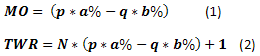
If we consider "heads or tails" in its most simple form, then we can calculate some things quite easily knowing the number of N bets. For example, mathematical expectation (МО) of revenue per one bet (1) or expected revenue for a series of bets (2). Note that МО is defined relative to the initial funds here. It means that we have positive expectation in case МО>0 and if МО<0, it is expected that each bet is loss-making on the average.

For the case mentioned in [9]: p=0.45, q=0.55, a%=0.08, b%=0.05, N=20, the results are MO=0.0085, TWR=1.170. This case is interesting in that with the probability of win p<0.5, МО remains positive at one bet and consequently a profit of ~17% to the initial funds is expected.

Warning: another MM method is examined in [9]. Therefore, the results will be different despite similar input data.

However, such an expectation is akin to the average across the board. It tells nothing about the probability of occurrence of some of the results depending on the number of winning bets complicating evaluation of risks. Therefore, let's introduce two more equations: for calculating profit for a certain amount of winning bets (3) and calculating probability of occurrence of a certain amount of winning bets in a series (4):

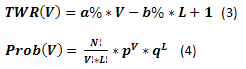
Now, we only have to calculate the values for all V= 0,1,...,N, L=N-V and create the graph of dependency of Prob(V) from TWR(V). For the previously described case, the graph looks as follows. Note that the graph displays Prob and TWR axes without (V) index. This has been done solely to make the graph look less complicated.

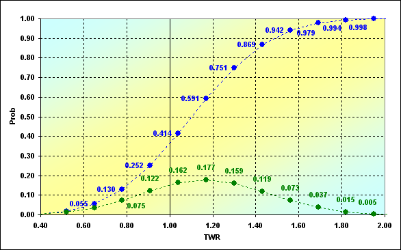
Fig. 1

Results of our calculations using equations (3) and (4) are shown as green dots. The graph can be interpreted as follows. For example, the probability of occurring the deals series results, in which TWR=1.04, is 0.162. Most often, with probability of 0.177, TWR=1.170 and so on. The blue dots represent the same data in the form of cumulative probability. Thus, the probability of loss (i.e., some of the game rounds have TWR<=1.00) for our input data comprises 0.252. Extreme values are not displayed on the graph. The case of ruin (TWR=0.00) has Prob=6.4E-06. Maximum gain TWR=2.60, - Prob=1.2E-07. These are very small probabilities. However, their existence creates another important issue.

Let's try to demonstrate this with the following example. Calculations have been performed for the following conditions: p=0.45, q=0.55, a%=0.05, b%=0.05, N=50. Results are displayed in the graph.

Fig. 2

As we can see, TWR takes on the values from -1.50 up to 3.50. TWR=-1.50 is possible only in case the game has been performed with the amount of funds less than 0.0. Thus, the equations we used do not consider the fact that the funds were depleted at one of the intermediary deals and the game could not be continued. Therefore, the new task has emerged, the so-called "boundary absorption issue". This issue considers that there is some boundary (or a limit) for the existing funds. When this boundary is reached, the game is stopped. In its simplest form, it is assumed that the boundary =0. However, we are more interested in the case when it can take on arbitrary values. Some aspects of the analytical solution of this issue are revealed in [7].

Range of Opportunities

Let's try to solve this problem numerically, first, by using iterative calculations, and second, using simulations modeling based on stochastic methods (Monte Carlo method). First of all, let's examine the figure and try to sort out the problem.

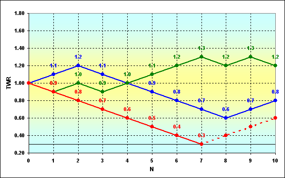
Fig. 3

The figure schematically displays possible change trajectories of the funds during the game. Three cases are displayed, though there are much more of them, of course. It is assumed that players having the funds that exceed, for example, 0.3 (collateral requirements) are allowed to participate in the game. Suppose that the game took the red course and it became impossible to continue playing. Boundary absorption of the trajectory has occurred meaning complete ruin. The player is dropped out of the game, unlike the games that took green or blue courses. Thus, we need to define the ruin probability at the previous steps in order to define it at some definite one.

The most simple, intuitive and very old technique that can be used to carry out such calculations is Pascal's triangle. In fact, this is a recursive procedure in which the next value is calculated using the previous ones. The slightly modified triangle is displayed below.

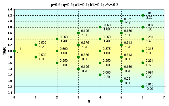
Fig. 4

Green dots indicate possible locations on the graph TWR trajectory can pass through. In this case, TWR can be calculated using equation (3). The dots have Prob values (numerator) and TWR values (denominator). z% symbol designates the boundary value at which absorption occurs (black line). The red horizontal line is drawn through z%+b% value.

What does location of dots relative to the red line represent? If the dot is located higher, the next round is possible. When the red line crosses the dot, this is the last chance for one more step. In case of success, the game continues, otherwise, absorption occurs. The dots between the red and black lines are achievable, but the next step out of them is impossible, as the funds are insufficient for the next bet. In other words, this is not a complete ruin but the game still cannot be continued.

Note: of course, this is not possible in case of integer bets, as when using coins, but if the bet is equal to, say, 0.15 of the funds, the overall picture is exactly like the one described above.

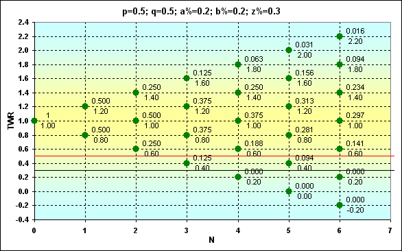
Fig. 5

Here is another figure containing calculation results in case of different boundary conditions. If we compare it with the previous one, we should be able to notice the difference.

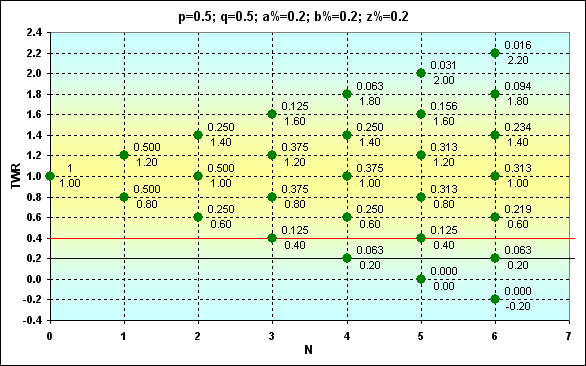
Fig. 6

Now, having such data, we are able to know the probability of any event. For example, what is Prob of TWR=1.4 in case of N=6 for Fig. 6? The answer is 0.234. Or what is Prob of TWR>1 in case of N=6? Corresponding Prob values should be summed. The answer is 0.344. Or what is Prob of TWR=1.1 in case of N=6? The answer is 0. And so on.

The last example of this series having "disfigured" input values: p=2/3, q=1/3, a%=0.1, b%=0.2, z%=0.2 is shown to demonstrate how Prob and TWR change in this case. As we can see, the win probability exceeds the loss one twice. However, the win size is half the size of a loss.

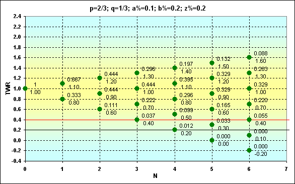
Fig. 7

If TWR>1, Prob=0.351. This Prob value is pretty close to the case displayed on Fig. 6. But it is clear that TWR values that can be achieved in a comparable number of bets are much less.

Another important thing that we have not discussed yet concerns f parameter indicating the share of funds involved in the bet. In fact, this is the share of the funds that are used in the deal, i.e. b%. In classic "heads or tails", it is possible to lose only a countable number of "coins". Thus, such an expression as 1/f displays the number of consecutive losses that leads to ruin. 1/f parameter may be non-integral in our case. At the same time, the number of bets cannot be non-integral considering non-divisibility of bets. It means that some part of the funds may still remain when the game cannot be continued (and this part will be less than b%). In other words, this part is absolutely risk-free, as it cannot be lost. In this regard, the actual amount of the funds participating in the game is less by this value. Thus, the actual z% parameter is larger by this value (see Fig. 5). In this case, if z%>0, then f tends to exceed b%. Considering all that, the actual f can be calculated the following way:

where int symbol stands for truncation. For the example displayed in Fig. 5, b%=1/5, but the actual f=1/3.

Duration of Opportunities

Let's consider our results to be a correspondence between Prob and TWR. Several different sets of input data have been selected as an example. All the series have the same length - N=15.

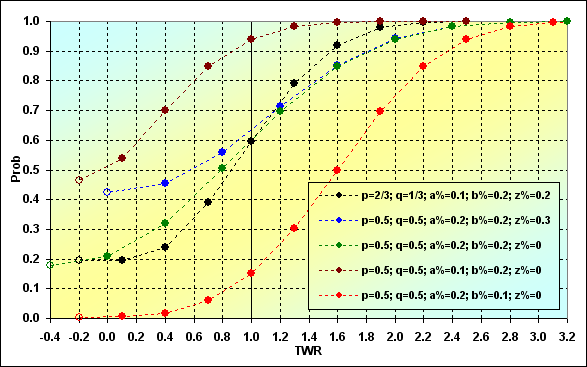
Fig. 8

Below are some explanations concerning what and how is displayed on the graph. Each curve starts with an "empty" dot (if we look from left to right). These are conditional points (in some cases), which may not exist actually. Nevertheless, they are applied indicating the probability of the absorption occurring on some of the intermediate steps. In other words, this is the probability of the trajectory not reaching the last step. The next dot on the graph represents actual data on the probability of the absorption occurring at the last step considering all previous ruins (with some exceptions that are not important here).

The next image demonstrates how the probability of ruin changes depending on N length of the series. The same input data as for Fig. 8 has been used for the example. As we will see further, the results are significantly different from each other.

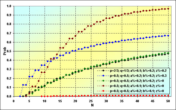
Fig. 9

The most important thing is that if the series length increases, so does the ruin probability. This key issue cannot be eliminated in case of a boundary absorption game. However, not everything is as bad as it seems at first glance. The probability of ruin can turn out to be very small depending on TS parameters (see the red line). If TS parameters are not very successful, the ruin occurs rapidly (see the brown line).

Another important issue is the probability of total win. We have already considered the case of TWR<(z%+b%), now it is time to define the TWR>1 probability behavior depending on N.

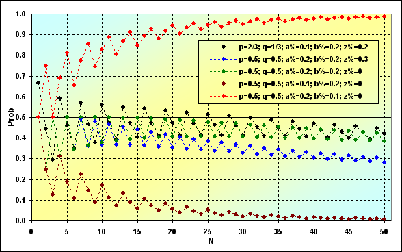
Fig. 10

In the case shown in green and black colors, we deal with neutral strategies, i.e. the ones having MO=0 and we have all reasons to expect that the win probability should be about 0.5. However, this is not the case. And that has to do with boundary absorption.

That is how the probability of possible TWR occurring at a certain step looks. In this case, N=50, which is similar to the Fig. 10 value.

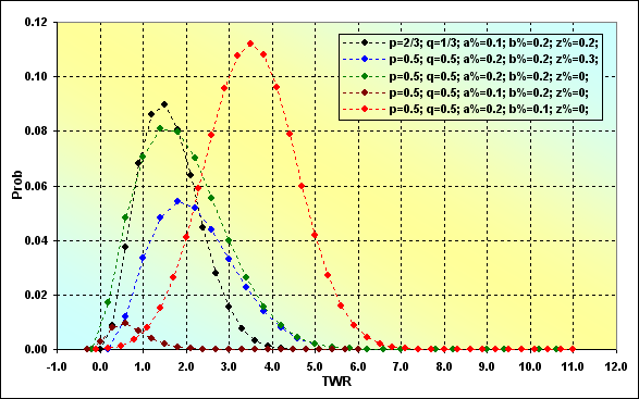
Fig. 11

These are ordinary distribution curves. Their difference from the conventional distribution curve is that they are asymmetric relative to their maximum value, as well as their minimum and maximum TWR. Besides, some curves are noticeably skewed and resemble lognormal curves. Another interesting moment is that if we compare Figures 10 and 11, we will see the following. While most distributions in Figure 11 have the most probable TWR value of more than 1, the probability of TWR value being more than 1 is less than 0.5. Moreover, for cases with MO=0 (black and green lines), the most probable TWR is also not equal to 1, as it could be expected. There is no paradox in that.

Now it is time to finish our brief review of some aspects of "boundary absorption task". The next thing we should do is to perform stochastic simulation and compare results with the previously obtained ones to evaluate the correctness of reasoning and simulation accuracy.

Simulation

In general, the following simulation algorithm is used. The amount of funds is checked before each "coin" toss. If the funds are insufficient to continue the game, it is stopped. If the game can be continued, PRNG is used to define if the bet was a winning or losing one. The funds are increased or decreased according to the results. The algorithm remains the same to the end of the game. The large amount of game rounds are performed, results are averaged. It is all very simple. The only problem of stochastic methods lies in their accuracy. When using this method, the accurate solution of the task is impossible to be found and that has been proven mathematically (see de Moivre paradox). Therefore, we should define to what extent the results are consistent with other ones before using this model in further calculations.

Let's compare two solution cases for the following parameters: p=0.5, q=0.5, a%=0.2, b%=0.1, z%=0.0. Below are two figures (12 and 13) displaying the correspondence of the results.

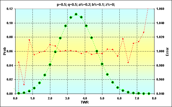
Fig. 12

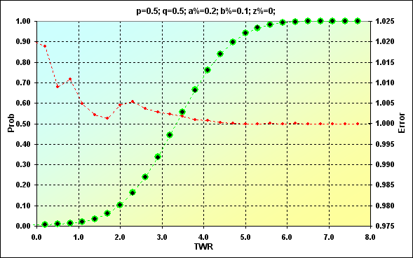
Fig. 13

Previously obtained values are shown in green. Black dots show simulation results. The red color represents the error, the ratio of the expected value to the simulation one. Figure 12 displays the values, while Figure 13 is an accumulated sum. The match is quite good. The error rate at the midpoint of the values is less than 0.5%. Of course, the error rate is higher at the edges of the range. However, there is nothing to worry about. We just should consider that in the future. Besides, we are more interested in the accumulated sum. The error rate is much less there (this is a feature of the cumulative curves when errors from different values cancel each other).

Another feature of the simulation results is that it is almost impossible to receive the probability of extremely rare values. In the above example, maximum TWR=11, while Prob= 8.88E-16. These values could not be obtained in simulation.

Another example that demonstrates the above mentioned fact in case of N=250: p=0.5, q=0.5, a%=0.1, b%=0.1, z%=0.0. No further comments are needed here.

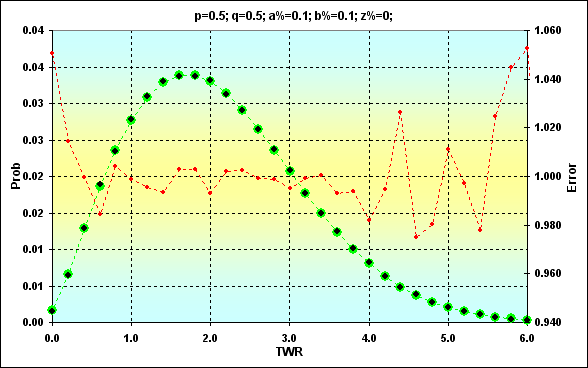
Fig. 14

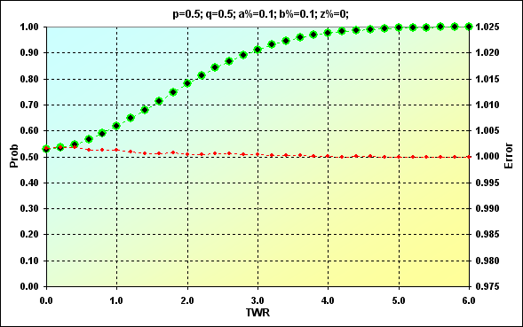
Fig. 15

Now we can use this model as a basis for solving the more complex problem than the one we considered above.

Trading Operations

Before we continue our discussion, I would like to focus on concepts and equations. At first glance, real trading is quite different from "heads or tails" game described above - considering this fact requires additional efforts during simulation. Therefore, it is necessary to clarify at once what we will have to deal with in the future. Of course, most readers have their own ideas about that. Below are some useful concepts and notations.

Note: for simplicity, only transactions with "direct quotation" pairs, such as EURUSD and GBPUSD, will be examined. "Indirect quotation" pairs and cross rates are calculated in a different way. For indirect quotation pairs, the point's price changes according to the current quote. For cross rates, the current quote of the base (first) currency to USD is additionally considered. Besides, ASK and BID concepts are not used here.

The funds used in trading will be called Deposit. We have the right to buy and sell contracts having a certain LotSize using Leverage. The contract may be fractional, so we need the concept of Lots as a parameter indicating the applied contract size. The actual size of the used lot in base currency will be called LotPrice accordingly. We should pay Margin for the right to buy or sell. If we express Margin as a share of Deposit, we will receive Margin% parameter. We will also use StopOut indicating the minimum part of Margin. Reaching it leads to closing of the current deal and the trading is stopped forcedly. Thus, there are two different situations when further trading is impossible (at the desired rate of LotPrice), i.e. the case of ruin. Another parameter Sigma has additionally been included. This is the ratio of the funds used in trading operations considering credit to equity. Ratio of the used funds to the actual capital, i.e. the analogue of a leverage, though it is applied to the entire Deposit instead of LotPrice.

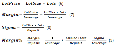
One of the basic concepts that characterize trading process is Quote - current exchange rate. Minimum rate change is Tick. The size of the symbol's rate minimum change is TickPrice considered as part of Deposit - Tick%.

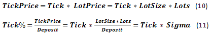
Besides, we have a few more parameters connected with rate change: the so-called TP (TakeProfit) and SL (StopLoss) - rate change, at which profit or loss is fixed. If we express these parameters in currency, they will be called TPprice and SLprice. The ones expressed as the part of Deposit will be called TP% and SL%. Also, there are various dealer commissions including Spread, Swap etc. We will not examine the entire diversity of these parameters focusing only on Spread, which is traditionally displayed in points of rate change. If necessary, Swap data can be considered quite easily if it is also displayed in points. If Swap is presented as an actual interest rate on borrowed funds used with the help of a leverage, the situation turns out to be somewhat more complicated.

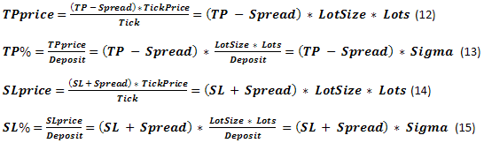
Let's compare obtained parameters with the ones used in "boundary absorption" problem. SL% clearly corresponds to b%, while TP% = a%. The initial funds have been presented as TWR=1. The current case is similar, as our calculations are based on parameters displayed in fractions of a unit. z%+b% boundary value can be conventionally considered as Margin%. There is some difference between these concepts but it is not so critical in case we do not consider the existence of StopOut. It appears that the tasks are similar at the first approximation. We will check this claim later.

If we closely examine the equations (9, 11, 13, 15), we will see Sigma parameter in all of them. As already mentioned, this is an equivalent of a leverage used in all critical equations. Leverage can directly affect only Margin%.

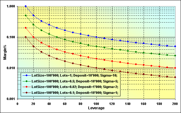
Fig. 16

Correctness of the calculations can be checked by the following example. Suppose that if Leverage=100, LotSize=100000, Lots=0.1, Deposit=10000, the margin size is 100. If we look at the appropriate (brown) graph, we will see that Margin%=0.01. In case Deposit=10000, we will receive 100.

Two features can be observed in the graphs: first, the larger Sigma value, the higher Margin%, in other words, the less free funds that can be used in trading. Second, decreasing Leverage value also increases Margin%. Let's examine Figure 9 where similar cases are addressed (blue and green lines). These cases differ only in z% value. It can be seen that increase of the boundary value also leads to an increase of the ruin probability under otherwise equal conditions.

Since there is no direct relationship between SL% and Leverage, let's examine how this parameter depends on Sigma and (SL+Spread).

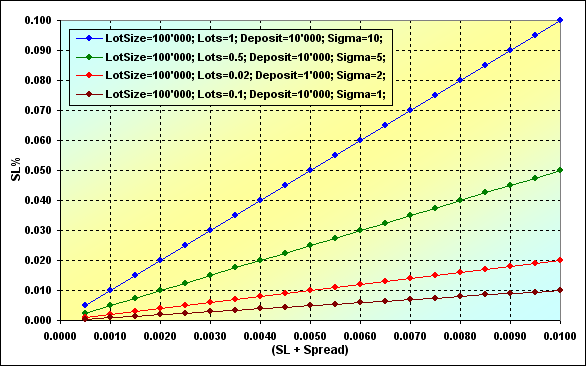
Fig. 17

Increase of Sigma parameter leads to increase of SL%. Thus, the ruin becomes much more probable again. This dependence is a linear one. It turns out that in order to decrease SL%, we need either decrease (SL+Spread) or Lots, since all other values included in Sigma most probably cannot be changed.

Then we are done with equations. Now, let's briefly describe how the simulation was conducted. The process is almost indistinguishable from the previous one. The possibility of trading has been checked, buy operation has been performed at the current market conditions, the rate has been determined with the help of PRNG, sell operation has been performed and the current funds level has been calculated. All this has been repeated multiple times in the loop. Trading results have eventually been defined. No specific analytical forms have been used, the entire simulation has been performed "as is". Tick and other related concepts, as well as Swap have not been used, as they have not been necessary.

In order to assess simulation results, we have used an example with the following basic parameters: Deposit=1000, Leverage=100, LotSize=100000, Lots=0.1, TP=0.0040, SL=0.0040, Spread=0.0002, p=0.5, N=250. The value of the series length is approximately equal to the number of working days per year. Thus, if we assume that one trade is performed per day (intraday deal, therefore, Swap is not used), results are annualized. After applying equations (9, 13, 15), we will receive the following results: TP%=0.038=a%, SL%=0.042=b%, Margin%=0.1 (thus, z%=0.058). Let's perform stochastic simulation and calculations similar to the ones displayed in Figure 4.

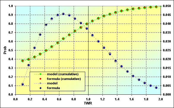
Fig. 18

Calculations based on the simulation and on the equations are compared here. As we can see, results of various calculations have a good match. This is another reason to claim that trading process is not much different from the classic "heads or tails" game when dealing with "boundary absorption" problem.

Below are a few brief comments on the graph. The left-most and the smallest dot of the green-red line displays the ruin probability. In our case, it is TWR<= Margin% - 0.375. The probability of loss is when TWR<=1, - 0.795, thus, the win probability is 0.205.

ММ - Fixed Size (FixSize)

The main idea of this MM method is that a fixed part of the initial funds is used each time despite any circumstances. In fact, conventional features of lot size management provided to traders by dealers directly correspond to this method. Besides, this method is implemented in "heads or tails" game. Since we have already covered the basic features of this method before, let's proceed to the issue of individual parameters affecting the system. We will use our model to tackle this issue.

As we consider numerical solution rather than analytical one, the only way to evaluate the effect of changes in the input parameters is to compare calculation results. We will fix the data, change some of the data in a certain range and observe the changes.

Let's return to the case displayed in Figure 16. Perform the calculations with the following parameters: Deposit=3000, LotSize=100000, Lots=0.1, TP=SL= { 0.0030, 0.0040, 0.0050, 0.0060}, Spread=0.0002, p=0.5, N=250, Leverage= { 3, 4, 5, 6, 7, 10, 25, 50, 75, 100}.

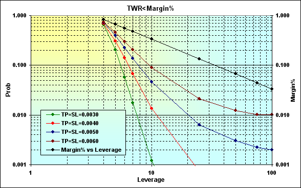
Fig. 19

Calculation results are shown on a logarithmic scale for greater clarity. Actually, decrease of Leverage leads to increase of Margin% (black line) enhancing the probability of ruin. The correlation between the ruin probability and the leverage is a non-linear one and its greatest impact can be felt in the area of small Leverage values. The negative effect caused by decreasing Leverage can be reduced by decreasing TP and SL levels. But even if Leverage value is small enough (in our case, it is 4), the ruin probability is still high enough. In addition, there is another feature that is displayed in the figure below.

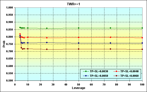
Fig. 20

The figure shows how the loss probability changes depending on altering Leverage value. As we can see, the loss becomes more probable when TP and SL decrease.

If we increase the funds up to, say, 10 000, the ruin becomes impossible in case of N=250. If we compare the figures 20 and 21, we will see that the results coincide in Leverage>10 area.

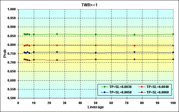
Fig. 21

Let's consider an example, in which the win probability in one deal is higher than the probability of loss, in other words, p>0.50. Perform the calculations with the following parameters: Deposit=3000, LotSize=100000, Lots=0.1, TP=SL={ 0.0030, 0.0040, 0.0050, 0.0060}, Spread=0.0002, p=0.52, N=250, Leverage={ 3, 4, 5, 6, 7, 10, 25, 50, 75, 100}.

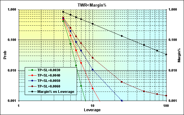
Fig. 22

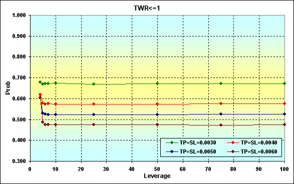
Fig. 23

If we compare calculation results displayed in Figure 19, we will see that increasing the gain per one deal decreases the ruin and loss probabilities. That is a natural and expected result.

The following example shows how win probability affects the loss one in one deal considering TP, SL level. The parameters are as follows: Deposit=3000, LotSize=100000, Lots=0.1, TP=SL={ 0.0020, 0.0030, 0.0040, 0.0050, 0.0060}, Spread=0.0002, p={ 0.48, 0.49, 0.50, 0.51, 0.52, 0.53, 0.54, 0.55, 0.56, 0.57}, N=250, Leverage=100.

Note: Example has been selected so that the ruin probability value is inconsiderable and can be disregarded. The highest ruin probability for the worst case comprises about 0.04.

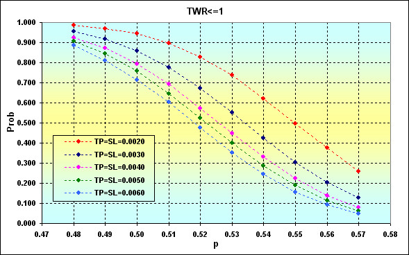
Fig. 24

The first important thing is that increase of p decreases the probability of loss. Decrease of TP and SL levels has the opposite effect. This happens due to fixed Spread value. Another conclusion that can be drawn from these results is that trading with low levels in each deal is quite a risky thing.

Example below demonstrates the extent to which Spread value affects the loss probability. Main parameters of the simulation: Deposit=3000, LotSize=100000, Lots=0.1, TP=SL={ 0.0020, 0.0030, 0.0040, 0.0050, 0.0060}, Spread={ 0.00000, 0.00005, 0.00010, 0.00015, 0.00020, 0.00025, 0.00030, 0.00035, 0.00040, 0.00045}, p=0.55, N=250, Leverage=100.

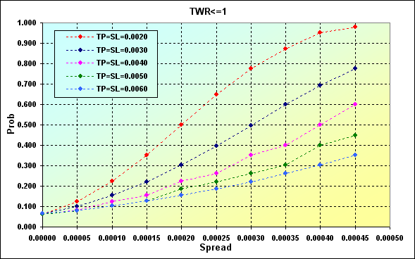
Fig. 25

The next figure demonstrates the correspondence between the loss probability and MO of the deal calculated by using equation (1) for the data displayed in Fig. 24. Instead of a% and b% values, the appropriate TP% and SL% ones have been used.

Fig. 26

As we can see, increase in MO of the deal reduces the loss probability, though it cannot be reduced to zero. It means that positive MO alone does not guarantee protection against loss, as well as ruin. Greater TP and SL levels certainly reduce the loss probability. But at the same time (see Figures 19 and 22), that increases the ruin probability.

In other words, we have again returned to our previous statement that I expressed when describing the classical "heads or tails" game. Increase in bets leads to an increase of possible gain (and reduces the loss probability), while making the ruin more probable. Unfortunately, no mathematically sound method of selecting a deal volume when applying this MM method exists. We can use only our personal preferences on what level of ruin or loss is acceptable in each case.

Let's consider the issue of determining the probability of reaching a certain TWR level during the game. Main parameters of the simulation: Deposit=3000, LotSize=100000, Lots=0.1, TP=SL= 0.0030, Spread=0.0002, p={ 0.48, 0.49, 0.50, 0.51, 0.52}, N=250, Leverage=100.

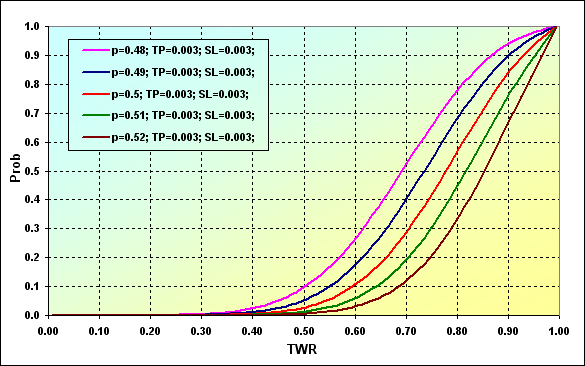
Fig. 27

Graph data can be interpreted the following way. The probability of TWR value decreasing down to ~0.90 in case of p=0.48 is ~0.93. If p=0.52, the value is ~0.68.

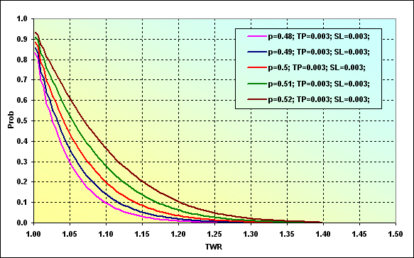
Fig. 28

This figure displays the probability of TWR level increase up to a certain value during the game. For example, the probability of TWR value reaching ~1.10 at p=0.48 is ~0.09. In case of p=0.52, the value is ~0.37. It is quite logical that increase of the win probability in one deal leads to increase in the probability of reaching a certain level.

Now, a few words about Drawdown. Script [10] with minor changes has been used to evaluate this parameter. Besides, unlike the original script, calculation is performed considering Spread.

Main parameters of the simulation: Deposit=3000, LotSize=100000, Lots=0.1, TP=SL=0.0030, Spread=0.0002, p={ 0.48, 0.49, 0.50, 0.51, 0.52}, N=250, Leverage=100.

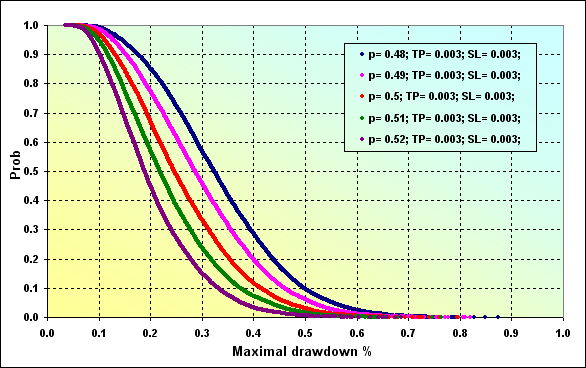
Fig. 29

In case of the initial parameters similar to Fig. 27, the probability of Maximal Drawdown % ~0.20 at p=0.48 is ~0.85. In case of p=0.52, the value is ~0.47.

The next and final example: Deposit=2000, LotSize=100000, Lots=0.1, TP=SL={ 0.0020, 0.0030, 0.0040, 0.0050, 0.0060}, Spread=0.0002, p=0.50, N=250, Leverage= 100.

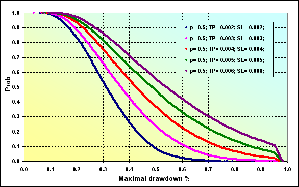
Fig. 30

One small note concerning Figure 30. Maximal Drawdown % level is 0.96 approximately matching Margin level. That is why we can see a sharp break in lines in the graphs. As we can see the probability of reaching greater Maximal Drawdown % values has increased, as compared to the case shown in Figure 29 (red line).

Before finishing our discussion on some features of MM having fixed size, let's examine two more distributions of such model characteristics as Profit Factor and Expected Payoff.

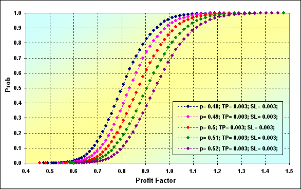
Fig. 31

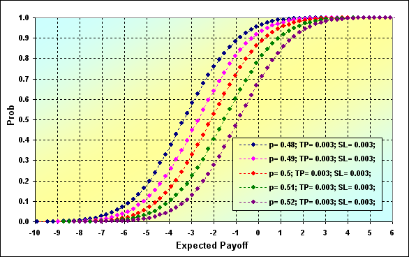
Fig. 32

Main parameters of the simulation for Figures 31 and 32: Deposit=3000, LotSize=100000, Lots=0.1, TP=SL= 0.0030, Spread=0.0002, p={ 0.48, 0.49, 0.50, 0.51, 0.52}, N=250, Leverage=100.

ММ - Fixed Fraction (FixFrac)

This method comprises ММ having a bet as a fixed fraction of the current funds. Share size is initially determined, for example, 10% for participating in deals. The amount of funds used in deals is calculated based on the current amount of the overall funds afterwards, regardless of the trading results. Thus, each successful deal increases the volume of the next one and vice versa. Sometimes, this system is called anti-martingale (though, strictly speaking, it is incorrect). This system assumes reinvestment of possible profit as opposed to MM having the fixed size.

Advantages and drawbacks of this MM method are well-known already. This method provides rapid growth of funds in case of successful deals. This growth has the form of a geometric progression as opposed to an arithmetic one in case of the fixed size method. In theory, this method prevents complete loss of funds in case of the infinite divisibility of bets (though this is not the case for real trading, of course).

One of the method's drawbacks is the so-called asymmetric leverage effect. It means that the next bet after the loss-making one has lesser volume. Thus, a player should have more successful deals than loss-making ones in order to recover the losses. Besides, hidden series in deal consequences may affect this method's results (non-Bernoulli).

During its practical use, this MM method may pose an issue of selecting the funds share that can provide the best funds growth rate combined with acceptable ruin probability. Such an asymptotically optimal game strategy has been offered by Kelly.

But first, let's examine some theory and equations. If we know the number of profitable and loss-making bets, as well as win and loss values per one bet, we can calculate TWR(V) and Prob(V) the same way as in case of the fixed size method. The equation (17) is similar to (4).

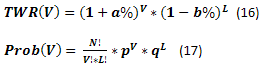
Example of calculation using equations (16) and (17) is displayed below. The probability of reaching different TWR values is shown as an accumulated value.

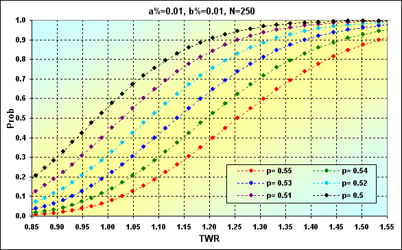
Fig. 33

The next figure shows the two cases with similar conditions but different MM. The fixed size case has been taken from Fig. 8. Fixed size MM (FixSize) is shown in red, while fixed fraction one (FixFrac) in black.

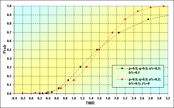
Fig. 34

The equation describing the speed of the funds growth in case of equal profit and loss values looks as follows.

By using simple transformations and reasoning [8] and minimizing expected average geometrical growth, we can produce the following equation showing the optimal f* bet size.

This is the so-called Kelly criterion. Its idea is quite simple. If you have a ТS with the win probability exceeding 0.5, while profit and loss values are equal, then you need to use the funds share calculated using equation (19) when placing a bet. For example, p=0.55, in this case, f*=0.55-0.45=0.10. It means that you need to use one tenth of the funds when placing a bet in order to make the funds grow efficiently.

Warning: please note that Kelly's optimal bet value equation is different from the one offered by Vince in [4]. There is no any mistake from Vince's side here and I will explain that later on.

Note: If we calculate optimal funds share value for p=0.50, then we will naturally get 0.00. In other words, it is recommended not to play at all.

In case profits and losses are k times different, we should use another equations instead of (18) and (19). [8][5].

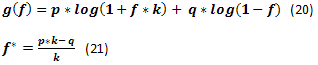
If we create g(f) change graph from f using equation (20), we will see something like the following figure. This figure is marked by f* point. This is the highest point of the graph where the funds growth rate reaches its maximum. Besides, there is fc point representing the intersection point of the graph and a zero line. It is the point where the funds growth rate is zero.

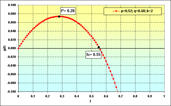
Fig. 35

Note: k=2 has been selected solely as an irony addressed to the appropriate graphs displayed in Vince's books. Nevertheless, such k value provides greater "clarity" and "beauty" to the methods he advocates.

In [8], it is stated that if the game is performed along the specified conditions, then f* provides maximum funds growth rate and zero ruin probability. If the share less than f* is used, ruin probability is also zero, though the funds growth rate is lower. If the used funds share exceeds fc, the ruin is imminent (in this case, any fund stock is meant as a ruin, no matter how low it is). If the funds occupy the range from f* to fc, growth rate is also slower than the maximum one, though there is no ruin probability.

The results are impressive enough. However, these theoretical calculations do not take some real world features into account. Therefore, Vince recommends to calculate the optimal fс with consideration to maximum losses. This leads to the fact that his f* value becomes lower than that calculated strictly mathematically with all ensuing consequences.

Let's try to consider how it may look on the graphs. Let's take the following case: Deposit=1000, LotSize=100000, f={ 0.01, 0.02, 0.03, 0.04, 0.05}, TP=SL=0.01, Spread=0.0000, p=0.51, N=250, Leverage= 100. With these input data, initial Lots=0.01, while TP%=SL%=0.01. Besides, f*=0.02 and fc=0.04, as shown in the following figure.

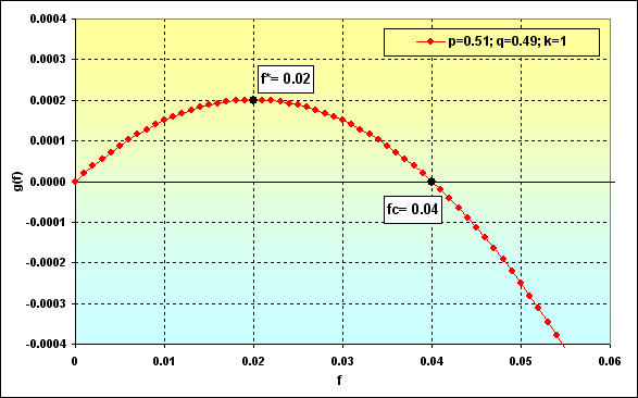
Fig. 36

In case of f changes, we will have the following correlations between Prob and TWR. Let's perform a few calculations to demonstrate this.

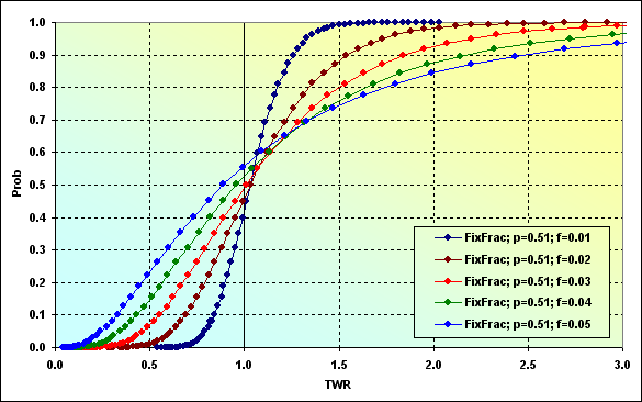
Fig. 37

Let's consider this in more detail. The line corresponding to f=0.01 demonstrates previously discussed case of f<f* when the funds growth rate is lower than the maximum possible one, while the ruin probability is zero. In this case, the probability of loss TWR<=1 is equal to ~0.40.

The next case, f=0.02 is the one when the share of the used funds is the optimal one. The loss probability is ~0.45. In other words, more than a half of game rounds are expected to be profitable.

Calculation version f*<f<fc, i.e. f=0.03. The loss probability is ~0.45. The ruin is impossible under the given game conditions. However, the values TWR can descend to are more significant than in the previous cases. Greater profits are also possible.

Now the loss probability is ~0.50, i.e. f=fc=0.04. It is stated that in this case, TWR will almost certainly fluctuate between 0 up to +infinity.

And the last case, f>fc. The loss probability is ~0.55. Very considerable gains are possible in that case, but all funds will be lost in the long (infinite) run and TWR will be reduced down to the level that can be classified as ruin.

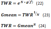
A little more equations. g(f) funds growth rate can be evaluated using equations (18) and (20). Since g(f) growth rate and the amount of deals N are known, it is possible to calculate TWR using the equation (22). Besides, it would be more correct to evaluate expected average profit from the deal for MM using fixed funds share as Gmean geometric mean using the equation (23) rather than arithmetic one.

Recommendation: It would be good to include the calculation of the deals' geometric mean to the MT tester's standard report. It would allow users to evaluate trading systems using fixed fraction MMs more correctly.

Below are two examples of calculation using the equations (23) and (24) and data from Figure 36.

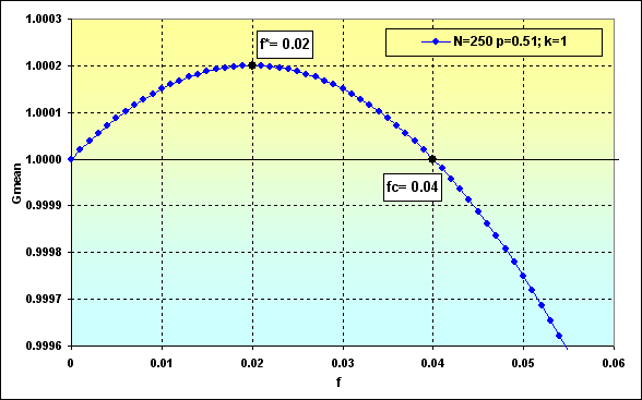
Fig. 38

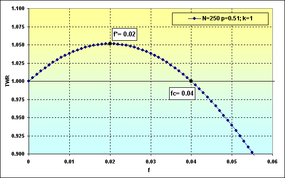
Fig. 39

Thus, based on Figure 39, the overall funds will tend to TWR=1.05 under the given conditions and with the optimal share in bets. As we can see in Figure 37, the probability of loss is ~0.45.

It would be interesting to know the behavior of different MMs having the same starting conditions. If we use data in Figure 36, we will see the following figure.

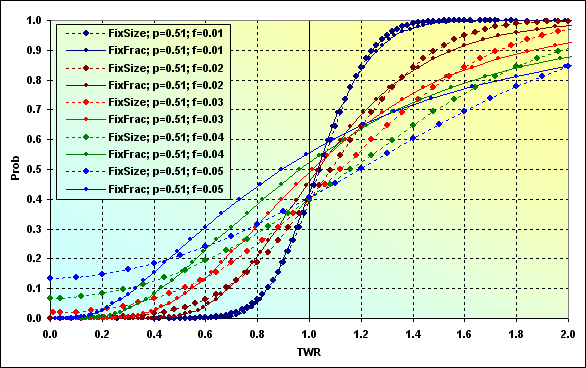
Fig. 40

In the case of f=0.01, charts are very similar, while MMs are different. In other words, the results can be similar under certain conditions. All other cases show that fixed size MM has lesser loss probability (TWR<=1) than fixed fraction one under the same starting conditions.

Warning: The above observation applies only to the selected input data. In no case it can be regarded as a general rule.

Let's show another interesting circumstance - a correlation of the values, to which TWR tends, with the funds share used in a deal. Calculation for these values can be performed for fixed size MM as multiplication of MO by N, while the equation (22) is used for the fixed fraction MM.

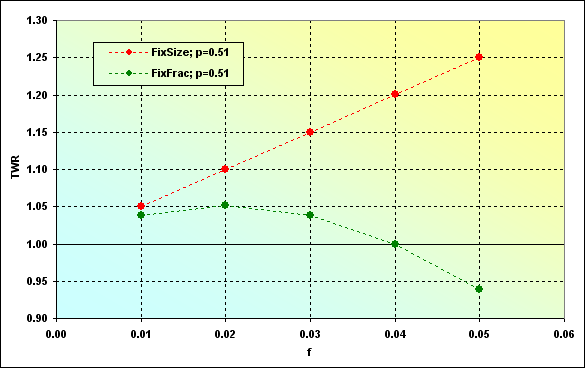
Fig. 41

As we can see, the expected payoff when using fixed size MM is higher (for the used input data). However, this is not always the case.

It is possible to examine how the correlations, to which TWR tends, change considering various win probabilities per one deal. The graphs for series length N=250 are shown below.

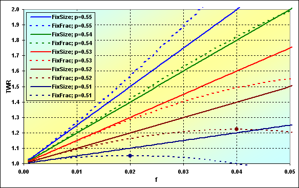
Fig. 42

As we can see, under certain conditions, in terms of the expected TWR, there may be situations when fixed size ММ is more preferable than fixed fraction one. However, if we consider this issue together with the ruin probability, the whole thing seems to be not so obvious.

Besides, the value of the expected TWR is significantly affected by N series length. In general, the longer the series, the greater the benefit of fixed fraction MM.

Now, let's finish our examination of some theoretical aspects and move on to simulation. In fact, nothing has changed in our initial model, besides the fact that it is necessary to add minimum and maximum lot concepts, MinLot and MaxLot. Besides, we will need LotStep value characterizing minimum possible step of the lot change. The general calculation algorithm remains the same. MinDeposit concept is initially introduced as minimum possible deposit value. Thus, trading can be continued if the deposit value exceeds Margin and MinDeposit.

Below is an example of simulating various MMs with the following input data. Deposit=1000, MinDeposit=300, LotSize=100000, MinLot=0.01, LotStep=0.01, MaxLot=100, f={ 0.01, 0.02, 0.03, 0.04, 0.05}, TP=SL=0.01, Spread=0.0000, p=0.54, N=250, Leverage=100. Please note that Spread is not used in this calculation.

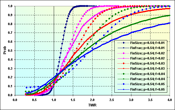
Fig. 43

Introduction of MinDeposit to calculations leads to the fact that fixed fraction ММ which had theoretically zero ruin probability (at f<fc) now has some non-zero one instead. Besides, discretization and lot size limitations also lead to ruin probability under some certain conditions (not displayed here). The impact of these negative factors can be reduced by taking the difference of Deposit and MinDeposit values as the initial funds. In fact, that is what Vince suggests - only a part of the funds should be used to calculate the optimal funds share. It seems to be a wise decision but it naturally leads to TWR decrease.

Now, let me make a few more clarifications concerning Figure 43. Let's find "FixFrac; p=0.54; f=0.05" on the graph where it corresponds to Prob=0.50. This is a median, the value, above and below which 50% of all values are located. In this case, it corresponds to TWR~2.00. In other words, half of all games has at least doubled the initial funds. The loss probability comprises ~0.20, while ruin probability is ~0.03. Comparing with "FixSize; p=0.54; f=0.05" graph, we can note that the ruin probability may increase up to ~0.08, while the loss probability decreases down to ~0.14, but the median approximately corresponds to TWR~2.00. If we are lucky to get to the number of cases where TWR>2.00, the result will most probably be lower than when using fixed fraction MM.

Comparing the graphs on Figures 42 and 43, we should note that Figure 42 values, to which TWR tends, are nothing else but the median in Figure 43.

Now, let's consider the case displayed in Figure 43 with Spread=0.0002. All other input data has remained the same.

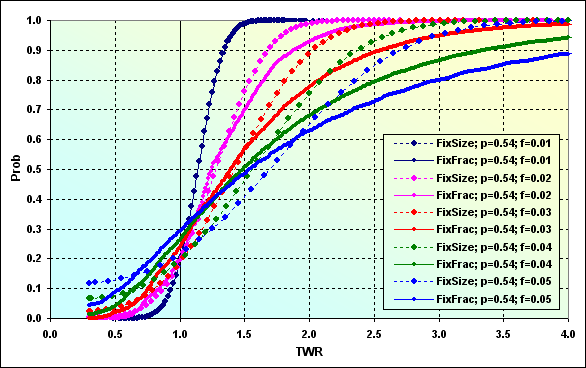
Fig. 44

As we can see, Spread comprising from 0.4% to 2% of the profit\loss level per deal leads to the considerable change of the entire picture. This can be best seen in the following figure where two calculation cases are compared (from Figures 43 and 44).

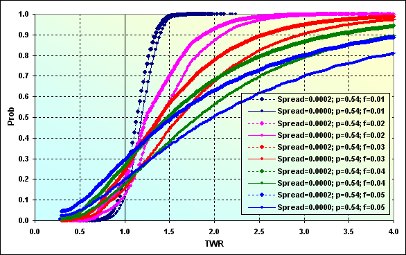
Fig. 45

Thus, Spread consideration decreases TWR median (for example, blue lines) from 2.00 down to 1.50. Loss probability has increased from 0.20 up to 0.30. The difference does not seem to be so large, only 0.10, but if treated differently, one in five players will lose (though not down to ruin) in the fist case, while it will be one in three players in the second one.

Let's try to examine how the loss probability changes affected by the win probability per one deal considering various f, simulating various ММs with the following input data: Deposit=1000, MinDeposit=300, LotSize=100000, MinLot=0.01, LotStep=0.01, MaxLot=100, f={ 0.01, 0.02, 0.03, 0.04, 0.05}, TP=SL=0.0100, Spread=0.0002, p={ 0.48, 0.49, 0.50, 0.51, 0.52, 0.53, 0.54, 0.55, 0.56, 0.57}, N=250, Leverage=100.

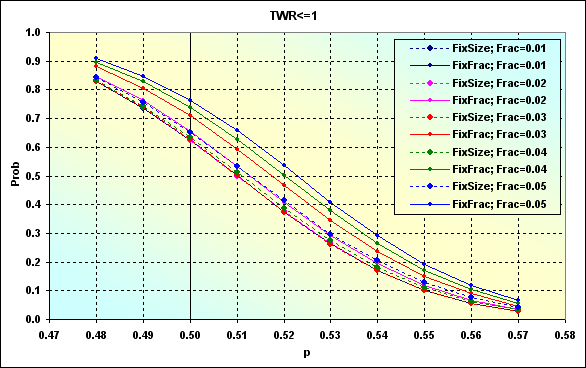
Fig. 46

This example differs from the one displayed in Figure 24 by the fact that TP and SL levels are fixed here but lot sizes are changeable. Figure 47 shows the case with the data similar to Figure 46 one at TP=SL=0.0050.

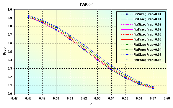
Fig. 47

Similar to the case displayed in Figure 24, decreasing TP and SL levels led to the loss probability increase. Besides, the scatter of values between various cases has decreased. The graphs have become "denser". In other words, affect of f value has decreased. This is particularly evident in the figure below.

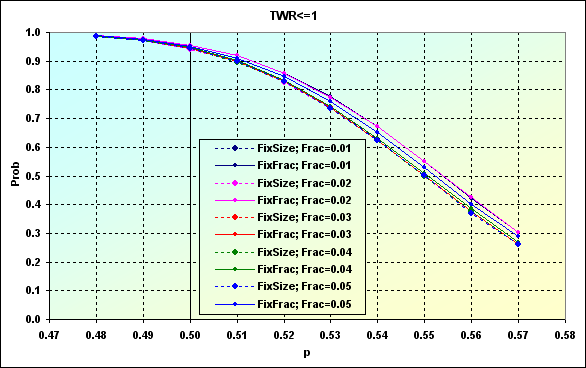
Fig. 48

TP=SL=0.0020 levels were used in this case. As we can see, in order to compensate Spread influence and reduce the loss probability down to less than 0.50, we will need a TS able to provide p=>0.56. But generally, if a TS can be profitable only in 50 cases out of 100 ones, results remain the same, the loss probability after 250 deals is ~0.95 regardless of MM type and f types.

Let's perform the calculation in order to show how TWR will look in case of TP=SL=0.0020 and p=0.56. The result is shown below. This is actually a case with the loss probability of about 0.40, as in Figure 48, while expected TWR value is 1.01...1.04. Different ММs display similar values.

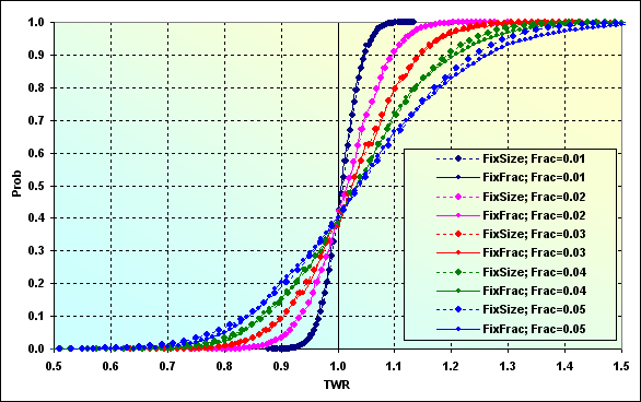
Fig. 49

As I have already mentioned, this is typical for cases with small levels. If Spread had been a floating value and had been charged as a percentage value of the bet size, the entire picture would have been different. That is exactly what happens on other markets other than "Forex for a wide range of customers".

Let's go back to the calculations with the following input data: Deposit=1000, MinDeposit=300, LotSize=100000, MinLot=0.01, LotStep=0.01, MaxLot=100, f={ 0.01, 0.02, 0.03, 0.04, 0.05}, TP=SL=0.0100, Spread=0.0002, p=0.51, N=250, Leverage=100. Let's consider how TWR decrease probability looks up to a certain level.

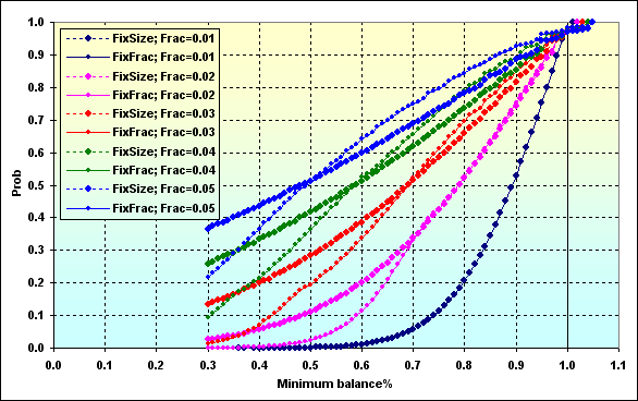
Fig. 50

The graphs' data should be interpreted the same way as in Figure 27. The probability of TWR value decreasing down to ~0.70 at f=0.05 is ~0.76 in case fixed fraction MM is used. If f=0.02, the value is ~0.34.

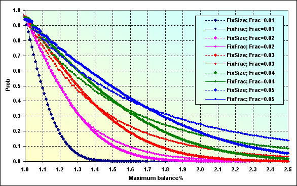
Fig. 51

And that is the probability of the deposit increase during the game for a certain value. This graph should be interpreted similar way as Figure 28.

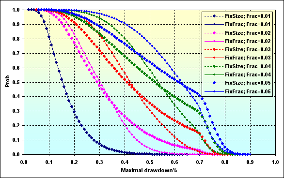
Fig. 52

The last graph displays Maximal Drawdown % probability of a certain value depending on the used funds share. Generally, we can assume that fixed fraction MM leads to larger Drawdown than when using a fixed size one. This can be explained by asymmetric leverage effect. Besides, if fc>f>f* is used, lesser Drawdown can be expected, while the profit may be similar to f<f* case.

Conclusion

We have examined two money management methods, reviewed their development backgrounds, as well as briefly learned about some theoretical aspects of the issue and a few simple equations. We have performed stochastic simulation research and evaluated obtained results comparing different methods. Perhaps, the most important conclusion that can be drawn from this study is that it is impossible to select the ultimate method out of the two examined ones. ММ's efficiency depends on a large amount of factors. Various combinations of these factors provide different results. Therefore, in each definite case, we should select the most appropriate MM depending on TS properties, dealing center conditions, as well as trader's possibilities and preferences. Our article has highlighted some possible solutions and crucial features. I hope that at least some traders have found this text useful. Good luck to all!

My future plans include examination of martingale (I think, that part will not take much time and space, as this method's properties are pretty obvious), as well as reviewing R. Jones' method (the author claims that it has been developed as a combination of advantages of the two examined MM methods).

References and web links (in order of appearance in the text)

1. Agner Fog - Pseudo random number generators - http://www.agner.org/random
2. strator - Probability Library (part of Cephes) - https://www.mql5.com/ru/code/10101 (in Russian)
3. Suvorov V. - MS Excel: Data Exchange and Management - https://www.mql5.com/en/code/8175
4. Vince R. - The Mathematics of Money Management.
5. Bershadsky А.V. - Research and Development of Risk Management Scenario Methods. - Dissertation, 2002 (in Russian).
6. Smirnov А.V., Guryanova Т.V. - On Ralph Vince's "optimal f" (in Russian).
7. W. Feller - An Introduction to Probability Theory and Its Applications.
8. E. Thorp - The Kelly Criterion in Blackjack, Sports Betting, and the Stock Market.
9. S. Bulashov - Statistics for Traders. (online version, p. 199, in Russian)
10. Starikoff S. - How to Evaluate the Expert Testing Results - https://www.mql5.com/en/articles/1403

Examples

Publicly available libraries used when writing this article are attached below. The scripts and the application are not attached. This has been done deliberately to stimulate development of trading server emulators among the members of MQL community. It was a trading server emulator that was used in simulation.

Disclaimers аkа Excuses

The author of this article bears no responsibility for anything. Complaints and suggestions are accepted in writing, in discussion section or via email. Sensible suggestions will be considered, while silly ones will be ignored. All copyrights are specified if known. Otherwise, the aurthor is unknown or the copyright has been lost.

The author admits that the text and calculations may contain inaccuracies or errors. The text is large and the subject is a complicated one, so errors are inevitable. Therefore, the author wanted to assign a $1 award for each detected fault similar to what D. Knuth did. But life has made some adjustments. The cold winds of the global financial crisis are still raging over the country. The most vulnerable and weakest among us - children left without parents - are usually the ones who suffer most at times like these. In order to help them, the author decided not to pay for his own mistakes but to spend the entire fee for charity. I have selected several orphan asylums in remote Russian provinces and sent my modest funds there.

It was an indescribable feeling when I received a response letter from the head of one of the orphanages. It was a simple letter written by hand on a sheet of paper from a squared copy-book. Of course, it contained words of gratitude but most importantly there was a list of purchased items. That wise woman spent the funds neither for a new computer to copy and paste letters of gratitude, nor for new curtains in her office, nor for food provided by the state, though it is much different from what people usually eat in Moscow. All the funds were invested into the education of those kids.

Copy-books, markers, pens, learning games, exercise-books, paints. All expendable materials that are so critical for the development of kids living in a small provincial town or village in an old wooden building possibly built by our ancestors who had just returned from the Great Patriotic War. So, if you can, if this is not your last money, please help them, do not be greedy or lazy. This will not go unnoticed. In fact, I'm not sure. Perhaps, that letter was written by a night watchman who was drinking away this unexpected gift. I'm not interested in that and I will never know the truth. I only made a bet, albeit a small one, that the probability of the fact that I live among normal people is much higher. Unlike heads or tails, this game is fair to all of us.