
Category Theory in MQL5 (Part 15) : Functors with Graphs
Introduction
In the previous article we looked at how concepts covered in prior articles like linear-orders, can be viewed as categories and why their ‘morphisms’ do constitute functors when relating to other categories. For this article we will expound on illustrations from the prior article by looking at how graphs can be of a similar use like linear-orders looked at in the previous article. To use graphs, we will reconstitute MQL5 calendar data as a graph, and thus as a category. This will be a key focus. The purpose of this article therefore, will like our previous one, seek to demonstrate the volatility forecasting potential of functors between two categories. In this case though, our domain category is a graph while the codomain will feature S&P 500 volatility values (not VIX) in a time series pre-order.
Reconstituting MQL5 Calendar Feed Data as a Graph
The MQL5 Economic Calendar was covered when we related category theory to database schemas so a re-introduction here of its relevance to traders is not pertinent. To represent it as a graph, a sequence of edges and nodes, firstly requires preselecting a subset of the news items we will include in our category. As is apparent from the economic calendar website there are a lot of items to choose from, however if we decide to select only say four based on a loose hypothesis that links them as shown in the diagram below:
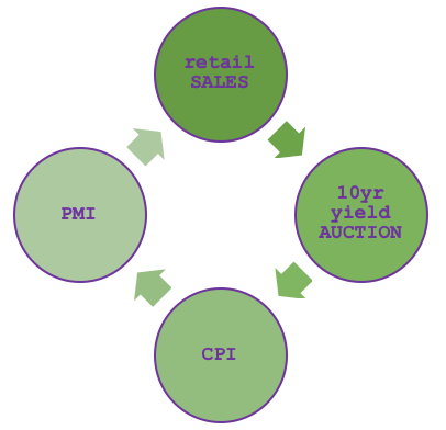
Then our hypothesis would be arguing that retail sales numbers are a function of producer PMI numbers, which in turn is derived from CPI, which in turn results from how well treasury auctions performed, which performance is also based on retail sales numbers. So, it’s a simple cycle whose veracity is not the subject of the article, but rather is meant to illustrate a possible graph composition from economic calendar data.
Graphs provide the benefit of simplifying complex interconnected systems by creating two straight forward tables, one of vertices’ pairings, and the other serving as an index of the vertices. A graph can be viewed as a category because the vertices can be seen as objects (domains) meaning the edges serve as morphisms. As a side note how this would differ from a linear-order looked at in the previous article is as the name suggests, in linearity. Graphs tend to accommodate more complex connections where an object/ domain can be connected to more than one object.
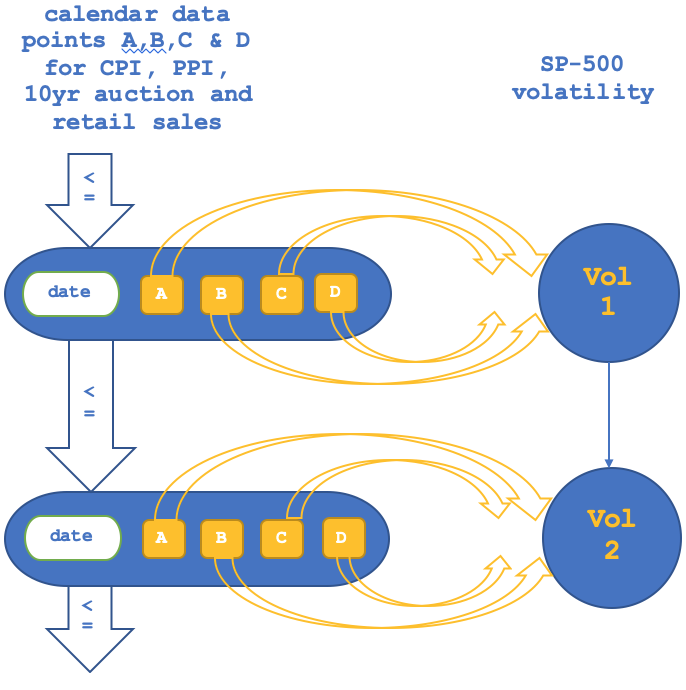
So rather than pairing individual objects in this category to objects in the S&P volatility category as we did in the previous article on linear orders, we will pair the rows of the vertex pairs to the S&P category. This implies it cannot be isomorphic as multiple rows are bound to pair to a single object (data-point) in the S&P given that the S&P is time based. It also means our domain objects will constitute four elements (the latest values of each of the four items in the cycle).
Category Theory and Functors recapped
Category theory has many applications as already mentioned in the articles this far but most public references tend to zero in on algebraic topology and this could be because of the original authors of this subject, which is why application to trading via MQL5 may seem novel. In fact, most traders that are familiar with MQL5 tend to use neural networks to develop an edge for their systems perhaps because they have been studied over a longer period compared to categories, well this should not deter exploring categories as well because the bottom line is most traders are seeking an edge and if a system or method is too common then the odds of finding one are lessened.
Functors, as already mentioned in our last article are effectively, morphisms between categories. These ‘morphisms’ do not just link the objects in two categories but they also connect the homomorphisms between the categories.
In the last article, we tested two scenarios one where we used the object linkage between two categories, and the other where we considered the morphism link between the same categories. A functor is a log of both, for our purposes though we explored the differences between the two by engaging one at a time and came up with strategy tester reports for each that highlighted relative importance in forecasting NASDAQ volatility. Given the short testing window of 1st January 2020 to 15th March the same year, conclusions on which mapping is better could not be drawn, but the difference in results indicated a high sensitivity and therefore about the need to emphasize one over the other.
Creating a Category of S&P 500 Volatility
The collection and processing of our SP500 volatility data will be straight forward and similar to the way we measured volatility for the NASDAQ in the last article. The VIX is a separate indicator to what we will be considering here, it is important readers note that. So, the current volatility reading will be recomputed on each new bar following the listing below:
      double _float_value=0.0;
      //where R is an instance of MqlRates...
      _float_value=(R.high-R.low)/Point();
As already mentioned the S&P will form our codomain with the objects capturing volatility values as one object sets and the morphisms between them capturing the relative change between the volatility readings. The initialization of this category could be handled as below:
//+------------------------------------------------------------------+
//|   Get SP500-100 data from symbol (NDX100 for this broker).       |
//|   Load it into SP500 category.                                   |
//+------------------------------------------------------------------+
void SetSP500(MqlRates &R)
   {
      _hmorph_sp500.Let();

      double _float_value=0.0;

      _float_value=(R.high-R.low)/Point();

      _element_value.Let();_element_value.Cardinality(1);_element_value.Set(0,DoubleToString(_float_value));
      _domain_sp500.Cardinality(1);_domain_sp500.Set(0,_element_value);

      //_category_sp500.Domains(_category_sp500.Domains()+1);
      _category_sp500.SetDomain(_category_sp500.Domains(),_domain_sp500);
   }
As seen in our last article if we can map a domain with a lag to this codomain, we could get some predictive ability on the volatility of the S&P 500. As in the last article we will test across object and morphism functors separately on identical signal and money management setups to gauge sensitivity.
Functors from Economic Calendar to S&P 500
We will construct the category of economic calendar data using the listing below:
//+------------------------------------------------------------------+
//|   Get Ocean data from file defined in input.                     |
//|   Load it into Ocean category.                                   |
//+------------------------------------------------------------------+
void SetEconomic(MqlRates &R)
   {
      datetime _time=R.time;

      int _elements=1;

      _e_retail.Let();
      SampleEvents(_time,_e_retail,IntToCountry(__country),__currency,TYPE_RETAIL_SALES);//printf(__FUNCSIG__+"...retail. ");

      _e_cpi.Let();
      string _cpi_time="";_e_retail.Get(0,_cpi_time);
      SampleEvents(StringToTime(_cpi_time),_e_cpi,IntToCountry(__country),__currency,TYPE_CPI);//printf(__FUNCSIG__+"...cpi. ");

      _e_auction.Let();
      string _auction_time="";_e_cpi.Get(0,_auction_time);
      SampleEvents(StringToTime(_auction_time),_e_auction,IntToCountry(__country),__currency,TYPE_AUCTION_10YR);//printf(__FUNCSIG__+"...auction. ");

      _e_pmi.Let();
      string _pmi_time="";_e_auction.Get(0,_pmi_time);
      SampleEvents(StringToTime(_pmi_time),_e_pmi,IntToCountry(__country),__currency,TYPE_PMI);//printf(__FUNCSIG__+"...pmi. ");

       _domain_economic.Cardinality(__ECON);
       _domain_economic.Set(0,_e_retail);
       _domain_economic.Set(1,_e_cpi);
       _domain_economic.Set(2,_e_auction);
       _domain_economic.Set(3,_e_pmi);

       _category_economic.SetDomain(_category_economic.Domains(),_domain_economic);
   }
Each object in this domain has two vertices which are the paired calendar values of which at least one is in the time range of the volatility value in the codomain. Since this economic data is released in intervals of approximately a month, we will test on the monthly timeframe. As in the previous article our functor mapping will have coefficients for each data point in the object. The difference here is we are faced with the possibility of multiple objects mapping to the same volatility in the codomain. Ideally, we will need to get the coefficient (for a linear mapping) from each object separately and use them in forecasting. This means they are bound to provide conflicting projections on top of those provided by the morphism mapping. This is why for the purpose of this article we could weigh each functor mapping from the calendar data to the S&P category and take the dot product sum of all to map to the volatility value.
Practical application of the functors as in previous article will follow two alternatives where we will map the objects in the first iteration and then we’ll map the morphisms in the next. The mapping of objects from ‘Output()’ function will be:
//+------------------------------------------------------------------+
//| Get Forecast value, forecast for next change in price bar range. |
//+------------------------------------------------------------------+
double GetObjectsForecast(MqlRates &R)
   {
      double _output=0.0;

      //econ init
      SetEconomic(R);

      //sp500 init
      SetSP500(R);

      matrix _domain;
      vector _codomain,_inputs;

      _domain.Init(__ECON+1,__ECON);

      for(int r=0;r<__ECON+1;r++)
      {
         CDomain<string> _d;_d.Let();
         _category_economic.GetDomain(_category_economic.Domains()-r-1,_d);

         for(int c=0;c<__ECON;c++)
         {
            CElement<string> _e; _d.Get(c,_e);

            string _s; _e.Get(1,_s);

            _domain[r][c]=StringToDouble(_s);
         }
      }

      _codomain.Init(__ECON);

      for(int r=0;r<__ECON;r++)
      {
         CDomain<string> _d;_d.Let();
         _category_sp500.GetDomain(_category_sp500.Domains()-r-1,_d);

         CElement<string> _e; _d.Get(0,_e);

         string _s; _e.Get(0,_s);

         _codomain[r]=StringToDouble(_s);
      }

      _inputs.Init(__ECON);_inputs.Fill(__constant_morph);

      M(_domain,_codomain,_inputs,_output,1);

      return(_output);
   }
Our morphism to morphism mapping will also be handled differently by mapping the morphisms between the vertices as defined by the change delta, to the morphism between the volatility data points of the S&P as also defined by the change value. This will be processed as follows:
//+------------------------------------------------------------------+
//|   Get Forecast value, forecast for next change in price bar range. |
//+------------------------------------------------------------------+
double GetMorphsForecast(MqlRates &R)
   {
      ...

      for(int r=0;r<__ECON+1;r++)
      {
         ...

         for(int c=0;c<__ECON;c++)
         {
            CElement<string> _e_new; _d_new.Get(c,_e_new);

            string _s_new; _e_new.Get(1,_s_new);

            CElement<string> _e_old; _d_old.Get(c,_e_old);

            string _s_old; _e_old.Get(1,_s_old);

            _domain[r][c]=StringToDouble(_s_new)-StringToDouble(_s_old);
         }
      }

      _codomain.Init(__ECON);

      for(int r=0;r<__ECON;r++)
      {
         ...

         CElement<string> _e_new; _d_new.Get(0,_e_new);

         string _s_new; _e_new.Get(0,_s_new);

         CElement<string> _e_old; _d_old.Get(0,_e_old);

         string _s_old; _e_old.Get(0,_s_old);

         _codomain[r]=StringToDouble(_s_new)-StringToDouble(_s_old);
      }

      _inputs.Init(__ECON);_inputs.Fill(__constant_morph);

      M(_domain,_codomain,_inputs,_output,1);

      return(_output);
   }
The diagrammatic representation of these two parts of the functor will also differ slightly from what we covered in the last article since our relation will no longer be isomorphic as was the case then. We can illustrate the object to object mapping as follows:
And that for morphism to morphism will look like this:

It is unfortunate MQL5’S strategy tester does not allow testing with access to economic calendar events. A lot of performance gains from developing a more robust trading systems are left on the table. So, since we have coded this as a script the best we can do is print the projected change to volatility based on our forecast and if you iterate through some history you can get a sense of how accurate our projections are.
None the less if we run our script that based price data provided by the broker we are able to construct our two categories from the graph of calendar data and from SP500’s volatility plus their connecting functor, we are able to get the following logs that make projections on volatility. The object to object functor mapping prints the logs:
2023.07.30 13:45:47.035 ct_15_w (SPX500,MN1)    void OnStart() Objects forecast is: 0.00000000, on: 2020.01.01 00:00, with actual being: 54260.00000000
2023.07.30 13:45:47.134 ct_15_w (SPX500,MN1)    void OnStart() Objects forecast is: 0.00000000, on: 2020.02.01 00:00, with actual being: 95438.00000000
2023.07.30 13:45:47.265 ct_15_w (SPX500,MN1)    void OnStart() Objects forecast is: 0.00000000, on: 2020.03.01 00:00, with actual being: 53588.00000000
2023.07.30 13:45:47.392 ct_15_w (SPX500,MN1)    void OnStart() Objects forecast is: 0.00000000, on: 2020.04.01 00:00, with actual being: 30352.00000000
2023.07.30 13:45:47.512 ct_15_w (SPX500,MN1)    void OnStart() Objects forecast is: 0.00000000, on: 2020.05.01 00:00, with actual being: 29694.00000000
2023.07.30 13:45:47.644 ct_15_w (SPX500,MN1)    void OnStart() Objects forecast is: -716790.11376869, on: 2020.06.01 00:00, with actual being: 21905.00000000
2023.07.30 13:45:47.740 ct_15_w (SPX500,MN1)    void OnStart() Objects forecast is: -12424.22112077, on: 2020.07.01 00:00, with actual being: 26509.00000000
2023.07.30 13:45:47.852 ct_15_w (SPX500,MN1)    void OnStart() Objects forecast is: 53612.17123096, on: 2020.08.01 00:00, with actual being: 37890.00000000


...

2023.07.30 13:45:50.294 ct_15_w (SPX500,MN1)    void OnStart() Objects forecast is: -27774.72154618, on: 2022.09.01 00:00, with actual being: 42426.00000000
2023.07.30 13:45:50.377 ct_15_w (SPX500,MN1)    void OnStart() Objects forecast is: 46751.59791572, on: 2022.10.01 00:00, with actual being: 39338.00000000
2023.07.30 13:45:50.487 ct_15_w (SPX500,MN1)    void OnStart() Objects forecast is: -19820.29385469, on: 2022.11.01 00:00, with actual being: 37305.00000000
2023.07.30 13:45:50.593 ct_15_w (SPX500,MN1)    void OnStart() Objects forecast is: -5370.60103622, on: 2022.12.01 00:00, with actual being: 30192.00000000
2023.07.30 13:45:50.700 ct_15_w (SPX500,MN1)    void OnStart() Objects forecast is: -4662833.98425755, on: 2023.01.01 00:00, with actual being: 25359.00000000
2023.07.30 13:45:50.795 ct_15_w (SPX500,MN1)    void OnStart() Objects forecast is: 33455.47933459, on: 2023.02.01 00:00, with actual being: 30681.00000000
2023.07.30 13:45:50.905 ct_15_w (SPX500,MN1)    void OnStart() Objects forecast is: -40357.22273603, on: 2023.03.01 00:00, with actual being: 12502.00000000
2023.07.30 13:45:51.001 ct_15_w (SPX500,MN1)    void OnStart() Objects forecast is: -37676.03496283, on: 2023.04.01 00:00, with actual being: 18835.00000000
2023.07.30 13:45:51.094 ct_15_w (SPX500,MN1)    void OnStart() Objects forecast is: -54634.02723538, on: 2023.05.01 00:00, with actual being: 28877.00000000
2023.07.30 13:45:51.178 ct_15_w (SPX500,MN1)    void OnStart() Objects forecast is: -35897.40757724, on: 2023.06.01 00:00, with actual being: 23306.00000000
2023.07.30 13:45:51.178 ct_15_w (SPX500,MN1)    void OnStart() corr is: 0.36053106 with morph constant as: 50000.00000000
While the morph to morph prints the logs:
2023.07.30 13:47:38.737 ct_15_w (SPX500,MN1)    void OnStart() Morphs forecast is: 0.00000000, on: 2020.01.01 00:00, with actual being: 54260.00000000
2023.07.30 13:47:38.797 ct_15_w (SPX500,MN1)    void OnStart() Morphs forecast is: 0.00000000, on: 2020.02.01 00:00, with actual being: 95438.00000000
2023.07.30 13:47:38.852 ct_15_w (SPX500,MN1)    void OnStart() Morphs forecast is: 0.00000000, on: 2020.03.01 00:00, with actual being: 53588.00000000
2023.07.30 13:47:38.906 ct_15_w (SPX500,MN1)    void OnStart() Morphs forecast is: 0.00000000, on: 2020.04.01 00:00, with actual being: 30352.00000000
2023.07.30 13:47:39.010 ct_15_w (SPX500,MN1)    void OnStart() Morphs forecast is: 0.00000000, on: 2020.05.01 00:00, with actual being: 29694.00000000
2023.07.30 13:47:39.087 ct_15_w (SPX500,MN1)    void OnStart() Morphs forecast is: -2482719.31391738, on: 2020.06.01 00:00, with actual being: 21905.00000000


...

2023.07.30 13:47:41.541 ct_15_w (SPX500,MN1)    void OnStart() Morphs forecast is: -86724.54189079, on: 2022.11.01 00:00, with actual being: 37305.00000000
2023.07.30 13:47:41.661 ct_15_w (SPX500,MN1)    void OnStart() Morphs forecast is: -126817.99564744, on: 2022.12.01 00:00, with actual being: 30192.00000000
2023.07.30 13:47:41.793 ct_15_w (SPX500,MN1)    void OnStart() Morphs forecast is: -198737.93199622, on: 2023.01.01 00:00, with actual being: 25359.00000000
2023.07.30 13:47:41.917 ct_15_w (SPX500,MN1)    void OnStart() Morphs forecast is: -280104.88246660, on: 2023.02.01 00:00, with actual being: 30681.00000000
2023.07.30 13:47:42.037 ct_15_w (SPX500,MN1)    void OnStart() Morphs forecast is: 24129.34336223, on: 2023.03.01 00:00, with actual being: 12502.00000000
2023.07.30 13:47:42.157 ct_15_w (SPX500,MN1)    void OnStart() Morphs forecast is: 4293.73674465, on: 2023.04.01 00:00, with actual being: 18835.00000000
2023.07.30 13:47:42.280 ct_15_w (SPX500,MN1)    void OnStart() Morphs forecast is: 763492.31964126, on: 2023.05.01 00:00, with actual being: 28877.00000000
2023.07.30 13:47:42.401 ct_15_w (SPX500,MN1)    void OnStart() Morphs forecast is: -30298.30836734, on: 2023.06.01 00:00, with actual being: 23306.00000000
2023.07.30 13:47:42.401 ct_15_w (SPX500,MN1)    void OnStart() corr is: 0.03400012 with morph constant as: 50000.00000000
A few points a worth noting from our log prints above. Firstly the first five months are all projecting a zero value. I think this is down to not enough price data to do complete computations as is sometimes the case with many indicators. Secondly negative values are part of the forecasts yet we are simply looking for a strictly positive value to indicate what our volatility will be on the next bar. This could be down to failing to size low volatility values since we are using the MQL5 library regression tools that use identity matrices in solving for our multiple coefficients (four). A walk around this could be by normalizing values that are negative via a function such as the one proposed below.
//+------------------------------------------------------------------+
//| Normalizes negative projections to positive number.              |
//+------------------------------------------------------------------+
double NormalizeForecast(double NegativeValue,double CurrentActual,double PreviousActual,double PreviousForecast)
   {
      return(CurrentActual+(((CurrentActual-NegativeValue)/CurrentActual)*fabs(PreviousActual-PreviousForecast)));
   }
If we now run our script and check for the correlation between our projections and the actual values, we are certainly bound to get different results especially since the equation constant is a very sensitive value that hugely determines what output, and projections we end up getting. We set it to zero for the logs generated below. First we run the object to object functor:
2023.07.30 14:43:42.224 ct_15_w_n (SPX500,MN1)  void OnStart() Objects forecast is: 15650.00000000, on: 2020.01.01 00:00, with actual being: 54260.00000000

...

2023.07.30 14:43:45.895 ct_15_w_n (SPX500,MN1)  void OnStart() Objects forecast is: 15718.63125861, on: 2023.03.01 00:00, with actual being: 12502.00000000
2023.07.30 14:43:45.957 ct_15_w_n (SPX500,MN1)  void OnStart() Objects forecast is: 12187.53007421, on: 2023.04.01 00:00, with actual being: 18835.00000000
2023.07.30 14:43:46.026 ct_15_w_n (SPX500,MN1)  void OnStart() Objects forecast is: 19185.80075759, on: 2023.05.01 00:00, with actual being: 28877.00000000
2023.07.30 14:43:46.129 ct_15_w_n (SPX500,MN1)  void OnStart() Objects forecast is: 11544.54076238, on: 2023.06.01 00:00, with actual being: 23306.00000000
2023.07.30 14:43:46.129 ct_15_w_n (SPX500,MN1)  void OnStart() correlation is: 0.46195608 with morph constant as: 0.00000000
And then we run our script while making projections based on the morphism to morphism functor, again with the same equation constant of zero.
2023.07.30 14:45:54.257 ct_15_w_n (SPX500,MN1)  void OnStart() Morphs forecast is: 54260.00000000, on: 2020.02.01 00:00, with actual being: 95438.00000000

...

2023.07.30 14:45:57.449 ct_15_w_n (SPX500,MN1)  void OnStart() Morphs forecast is: 257937.92970615, on: 2023.05.01 00:00, with actual being: 28877.00000000
2023.07.30 14:45:57.527 ct_15_w_n (SPX500,MN1)  void OnStart() Morphs forecast is: 679078.55629755, on: 2023.06.01 00:00, with actual being: 23306.00000000
2023.07.30 14:45:57.527 ct_15_w_n (SPX500,MN1)  void OnStart() correlation is: -0.03589660 with morph constant as: 0.00000000
We get a slightly higher correlation of 0.46 versus the 0.3 number we got without normalization. This could indicate some benefits from normalisation but in our case the input constant was changed from 50000, and as mentioned the forecasts and therefore correlation are very sensitive to it. So proper strategy tester runs, since we have just the one input, could be done to optimize this value and get more meaningful results.
Implications for Traders
An overlooked value of category theory to financial analysis in my opinion is transfer learning. The link just shared takes you to Wikipedia for an intro but what could not be easily inferred is the benefits we would get from our applications here. From our tests above, we came up with coefficients between the object functor mapping and the morphism mapping. The process of coming up with these coefficients is bound to be compute intensive especially if optimizing is done, as one would ideally expect, over long historical periods in MQL5’s strategy tester.
And yet because the functor coefficients are part of a set hypothesis, that was put forward above as a cycle, it can be argued that these coefficients which are working in a specific way for USD currency values from the economic calendar, could be just as effective on say EUR economic calendar values on EURO-STOXX volatility, or GBP values on FTSE volatility. This does present a list of possible combinations and where our functors become invaluable is in the use of coefficients attained from one lengthy compute intensive optimization, and applying them to any one of these alternatives which on paper based on our hypothesis could yield better than average results.
To illustrate this, using the inputs shown below:
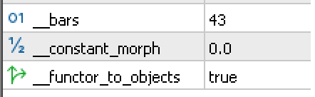
Let’s run a few tests with alternate currencies and their respective equity indices. If we start with the EUR economic calendar values as got from Germany in a category paired by functor to the DAX30 volatility category, then with the settings we have above we get tester report below:
2023.07.30 15:12:25.655	ct_15_w_n (GER30,MN1)	void OnStart() Objects forecast is: 75550.00000000, on: 2020.01.01 00:00, with actual being: 210640.00000000
2023.07.30 15:12:25.727	ct_15_w_n (GER30,MN1)	void OnStart() Objects forecast is: 210640.00000000, on: 2020.02.01 00:00, with actual being: 431320.00000000

...

2023.07.30 15:12:28.445	ct_15_w_n (GER30,MN1)	void OnStart() Objects forecast is: 144734.23693128, on: 2022.09.01 00:00, with actual being: 154697.00000000
2023.07.30 15:12:28.539	ct_15_w_n (GER30,MN1)	void OnStart() Objects forecast is: 171908.69769099, on: 2022.10.01 00:00, with actual being: 156643.00000000
2023.07.30 15:12:28.648	ct_15_w_n (GER30,MN1)	void OnStart() Objects forecast is: 298789.42486333, on: 2022.11.01 00:00, with actual being: 99044.00000000
2023.07.30 15:12:28.753	ct_15_w_n (GER30,MN1)	void OnStart() Objects forecast is: 178962.89317906, on: 2022.12.01 00:00, with actual being: 137604.00000000
2023.07.30 15:12:28.901	ct_15_w_n (GER30,MN1)	void OnStart() Objects forecast is: 440957.33259197, on: 2023.01.01 00:00, with actual being: 55544.00000000
2023.07.30 15:12:29.032	ct_15_w_n (GER30,MN1)	void OnStart() Objects forecast is: 143198.91357580, on: 2023.02.01 00:00, with actual being: 124659.00000000
2023.07.30 15:12:29.151	ct_15_w_n (GER30,MN1)	void OnStart() Objects forecast is: 24327.24201304, on: 2023.03.01 00:00, with actual being: 48737.00000000
2023.07.30 15:12:29.267	ct_15_w_n (GER30,MN1)	void OnStart() Objects forecast is: 167059.32862279, on: 2023.04.01 00:00, with actual being: 69888.00000000
2023.07.30 15:12:29.357	ct_15_w_n (GER30,MN1)	void OnStart() Objects forecast is: 67301.73632062, on: 2023.05.01 00:00, with actual being: 74073.00000000
2023.07.30 15:12:29.470	ct_15_w_n (GER30,MN1)	void OnStart() Objects forecast is: 87406.10063493, on: 2023.06.01 00:00, with actual being: 104992.00000000
2023.07.30 15:12:29.470	ct_15_w_n (GER30,MN1)	void OnStart() correlation is: 0.02260757 with morph constant as: 0.00000000
For GBP and the FTSE-100, we have:
2023.07.30 15:12:45.341	ct_15_w_n (UK100,MN1)	void OnStart() Objects forecast is: 45860.00000000, on: 2020.01.01 00:00, with actual being: 109780.00000000
2023.07.30 15:12:45.381	ct_15_w_n (UK100,MN1)	void OnStart() Objects forecast is: 109780.00000000, on: 2020.02.01 00:00, with actual being: 210420.00000000
2023.07.30 15:12:45.420	ct_15_w_n (UK100,MN1)	void OnStart() Objects forecast is: 210420.00000000, on: 2020.03.01 00:00, with actual being: 87250.00000000
2023.07.30 15:12:45.466	ct_15_w_n (UK100,MN1)	void OnStart() Objects forecast is: 87250.00000000, on: 2020.04.01 00:00, with actual being: 58380.00000000
2023.07.30 15:12:45.508	ct_15_w_n (UK100,MN1)	void OnStart() Objects forecast is: 1581489.63705309, on: 2020.05.01 00:00, with actual being: 58370.00000000

...

2023.07.30 15:12:46.685	ct_15_w_n (UK100,MN1)	void OnStart() Objects forecast is: 153576.16806574, on: 2023.01.01 00:00, with actual being: 30453.00000000
2023.07.30 15:12:46.710	ct_15_w_n (UK100,MN1)	void OnStart() Objects forecast is: 222058.94934174, on: 2023.02.01 00:00, with actual being: 77051.00000000
2023.07.30 15:12:46.739	ct_15_w_n (UK100,MN1)	void OnStart() Objects forecast is: 50993.02046828, on: 2023.03.01 00:00, with actual being: 30780.00000000
2023.07.30 15:12:46.784	ct_15_w_n (UK100,MN1)	void OnStart() Objects forecast is: 66795.26430874, on: 2023.04.01 00:00, with actual being: 45453.00000000
2023.07.30 15:12:46.832	ct_15_w_n (UK100,MN1)	void OnStart() Objects forecast is: 75492.86146563, on: 2023.05.01 00:00, with actual being: 28845.00000000
2023.07.30 15:12:46.876	ct_15_w_n (UK100,MN1)	void OnStart() Objects forecast is: 92298.50964858, on: 2023.06.01 00:00, with actual being: 49472.00000000
2023.07.30 15:12:46.876	ct_15_w_n (UK100,MN1)	void OnStart() correlation is: 0.14415363 with morph constant as: 0.00000000
It is clear from our initial logs, even though we are able to make projections, we cannot credibly verify them thanks to the limited use of calendar data in strategy tester. Clearly our hypothesis has not held and quite frankly the 0.46 correlation got above for USD and SP500 was hardly definitive.
In fact the correlation value is a temporary ‘solution’ since it only serves as a very early indicator to how reliable the forecasts are or could be depending on the choice of input, which in our case is chiefly one the coefficient of the linear relationship between the domain category and its codomain. Long term and more dependable options would involve manually exporting this economic calendar data either as a csv file to be read by an expert advisor or may be even to a database for better safe keeping. With either option one is able to conduct proper tests over the ideal long periods.
Besides forecasting volatility as a means of determining one’s ideal stop loss you could want to have a systematic approach to position sizing as well. To achieve this, with our methodology, suppose you have an unbound category of time series data that is the trade history of a particular security, where each object in the category represents a specific trade result, and the arrows (morphisms) between the objects represent changes to these results as logged through time.
To use this category in setting or forecasting the ideal position size for a trade system we would map this by functor to another category of a time series of ideal position sizes based on actual trade results, and perhaps the volatility that ensued. So, for instance if the trade was a loss then the object at that time, in the category would log a small position size, where as if it was accurate it would log a larger size. The volatility could serve as an extra factor to how much smaller or larger a position is depending on the volatility logged during the trade. So, the scaling could be such that when trades are losses the ideal position size is scaled down even more in proportion to the volatility reading. Likewise, if the trade result is a win then the ideal position size is also scaled up more again in proportion to volatility. The mapping functor would as expected have a lag such that say a trade result now is linked to a position sizing for the next period.
The functor would be linking not just trade results to anticipated ideal position size, but also the morphisms between the trade results to the morphisms between the ideal position size. As we’ve seen in the past article and also above, one can check the other, but a more insightful question could be how does the mapping function link the domain to the codomain.
Thus far we have used very basic coefficients based on regression from past results. As you can see from the attached source at the end of this article and the previous article, we assumed a simple constant plus a coefficient to the domain value were added to get the codomain value in what one could interpret as a simple linear relationship. But besides a linear relationship the domain values could be mapped to the codomain via a quadratic relation where, if our highest exponent is two, then we have an extra coefficient that gets multiplied to the domain value squared in order to arrive at the linked codomain counterpart. And of course, the more exponents one uses the more coefficients he will need in defining the functor map.
An alternative though to this simple and arguably error prone approach could be to have an artificial neural network define the homomorphism mapping between the two domains. This would have to be done for both the objects and the morphisms and is bound to yield more accurate results from training over large amounts of data for the most part; but the accuracy question aside it is intuitively the right approach since neural networks are adept at taking multiple inputs and producing a single output as would applicable in this case.
Conclusion
In summary, the main points covered here were composing economic calendar data as a graph, viewing this graph as a category, and like in our previous article using a functor relationship that is lagged to the volatility of the S&P 500 to make forecasts on the volatility of the S&P 500. We use these projections to move trailing stops of open positions as has been the case in these series. Besides adjusting the stop loss of open positions, we could use the functor relationship to set the position size of new orders or even define the entry signal for any tradeable security. These series are refraining from these last two examples in as far as assembling an expert advisor with the IDE wizard is concerned as I feel the reader is in a better position to fine tune these concepts to his own strategy. What we have also gleaned over this far has been the definition of morphing and now functor relations. We have been using crude incremental values that could have a linear or quadratic relation from domain to codomain but artificial neural networks could be used in defining this mapping as well. We could look into that in the next article(s).
- Free trading apps
- Over 8,000 signals for copying
- Economic news for exploring financial markets
You agree to website policy and terms of use