Description of architecture and implementation principles

Previously discussed types of neural networks operate with a predetermined volume of data. However, when working with price charts, it is difficult to determine the ideal size of the analyzed data. Different patterns may manifest over various time intervals, and these intervals are not always static, varying depending on the current market situation. Some events may be infrequent in the market but are likely to have a significant impact. Ideally, such an event should stay within the analyzed window. However, once it falls outside of it, the neural network no longer considers this event, even though the market may be reacting to it at that moment. Increasing the analyzed window leads to increased consumption of computational resources, requiring more time for training such a neural network. In practical real-world applications, more time will be needed for decision-making.

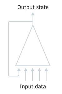
The use of recurrent neurons in neural networks has been proposed to address this issue in working with time series data. This involves attempting to implement short-term memory in neural networks, where the neuron input includes information about the current state of the system and its previous state. This approach is based on the assumption that the neuron output considers the influence of all factors, including its previous state, and passes all its knowledge to its future state on the next step. This is similar to human experience, where new actions are based on actions performed earlier. The duration of such memory and its impact on the current state of the neuron will depend on the weights.

Any architectural solution for neurons can be used here, including the fully connected and convolutional layers we discussed earlier. We simply concatenate two tensors: one for the input data and one for the results of the previous iteration, and feed the resulting tensor into the neural layer. At the beginning of the neural network operation, when there is no tensor of results from the previous iteration yet, the missing elements are filled with zeros.

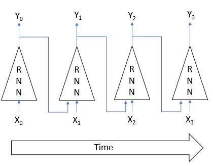
Training recurrent neural networks is done using the well-known method of backpropagation of errors. Similar to convolutional neural network training, the temporal nature of the process is unfolded into a multilayer perceptron. In such a perceptron, each time segment plays the role of a hidden layer. However, all layers of this perceptron use a single matrix of weights. Therefore, to adjust the weights, we take the sum of the gradients for all layers and count the delta of the weights once for the sum of all gradient layers.

Unfortunately, such a simple solution is not free from drawbacks. This approach saves "memory" for a short time. The cyclical multiplication of the signal by a coefficient less than one, combined with the application of the neuron activation function, leads to a gradual attenuation of the signal as the number of such cycles increases. To solve this problem, Sepp Hochreiter and Jürgen Schmidhuber proposed the use of the Long short-term memory LSTM architecture in 1997). Today, the LTSM algorithm is considered one of the best for solving classification and time series prediction problems, where significant events are separated over time and stretched over time intervals.

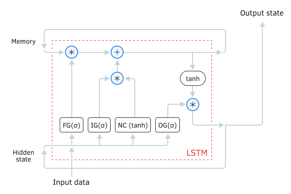
LSTM can hardly be called a neuron. Rather, it is already a neural network with three input data channels and three output data channels. Out of them, only two channels are used for data exchange with the surrounding world (one for input and one for output). The other four channels are locked in pairs for looping (Memory for memory and Hidden state for hidden state).

Within the LSTM block, there are two main information threads that are interconnected by four fully connected neural layers. All neural layers contain the same number of neurons, which is equal to the size of the output thread and the memory thread. Let's take a closer look at the algorithm.

The Memory data thread serves to store and transmit important information over time. Initially, it is initialized with zero values and filled during the neural network operation. One can compare it to a living person who is born without knowledge and learns throughout life.

The Hidden state thread is designed to transmit the system output state over time. The size of the data channel is equal to the data channel of the memory.

The Input data and Output state channels are designed to exchange information with the outside world.

Three threads of data enter the algorithm:

• Input data describes the current state of the system.
• Memory and Hidden state are obtained from the previous state.

At the beginning of the algorithm, information from Input data and Hidden state are combined into a single data set, which is then fed to all four latent LSTM neural layers.

The first neural layer, the Forget gate, determines which information stored in memory can be forgotten and which should be remembered. It is organized as a fully connected neural layer with a sigmoid activation function. The number of neurons in the layer corresponds to the number of memory cells in the Memory thread. Each neuron in the layer receives a total array of Input data and Hidden state data at the input and outputs a number between 0 (completely forget) and 1 (save in memory). The element-wise product of the output from the neural layer with memory flow returns the corrected memory.

where:

• σ = activation logistic function
• WFG = weights matrix for the input vector
• INPt = input vector for the current iteration
• UFG = hidden state weight matrix
• HSt-1 = hidden state vector from the previous iteration

In the next step, the algorithm determines which of the newly acquired information at this stage needs to be stored in memory. Two neural layers are used:

• New Content: a fully connected neural layer with hyperbolic tangent as an activation function normalizes the received information between −1 and 1.

• Input gate: a fully connected neural layer with a sigmoid as an activation function. It is similar to the Forget gate and determines what new information to remember.

The use of the hyperbolic tangent as an activation function for the neural layer of new content allows the separation of the received information into positive and negative. The element-wise work of New Content and Input gate determines the importance of the information received and the extent to which it needs to be stored in memory.

The vector of values obtained as a result of operations is element-wise added to the current memory vector. This results in an updated memory state, which is subsequently transmitted to the input of the next iteration cycle.

After updating the memory, we generate output thread values. To do this, normalize the current memory value using hyperbolic tangent. Similar to Forget gate and Input gate, let’s compute Output gate (the output signal gate), which is also activated by the sigmoid function.

The element product of the two received data vectors gives an array of output that is produced from the LSTM to the outside world. The same data set will be passed to the next iteration cycle as a hidden state thread.

Since the introduction of the LSTM unit, there have appeared many different modifications to it. Some tried to make it "lighter" for faster information processing and training. Others, on the contrary, made it harder to try to get better results. The GRU (Gated Recurrent Unit) model introduced by Kyunghyun Cho and his team in September 2014 is considered to be one of the most successful variations. This solution can be considered a simplified version of the standard LSTM unit. In it, the Forget gate and the Input gate are combined into a single update gate. This eliminates the use of a separate memory thread. Only the Hidden state is used to transmit information through time.

At the beginning of the GRU algorithm, as in LSTM, the refresh and reset gates are defined. The mathematical formula for calculating values is similar to the definition of the gate values in LSTM.

Then the current memory state is updated. In this process, the hidden state from the previous iteration is first multiplied by the corresponding weight matrix and then element-wise multiplied by the value of the reset gate. The resulting vector is added from the product of the raw data to its weight matrix. The total vector is activated by a hyperbolic tangent.

In conclusion of the algorithm, the hidden state from the previous iteration is element-wise multiplied by the value of the update gate, while the current memory state is multiplied by the difference between one and the value of the update gate. The sum of these products is passed as the output from the block and as the hidden state for the next iteration.

Thus, in the GRU model, the reset gate controls the rate of data forgetting. The update gate determines how much information to take from the previous state and how much of the new data.