Pan PrizMA
- Indicadores
- Aleksey Panfilov
- Versão: 1.3
- Atualizado: 23 março 2020
- Ativações: 20
The indicator builds a moving line based on interpolation by a polynomial of 1-4 powers and/or a function consisting of a sum of 1-5 sine curves. Various combinations are possible, for example, a sum of three sine curves about a second order parabola. The resulting line can be extrapolated by any of the specified functions and for various distances both as a single point at each indicator step (unchangeable line), and as a specified (re-painted) function segment for visualization.
More details: https://www.mql5.com/en/market/product/18363#!tab=comments
The indicator involves four lines. Each successive indicator line is based on the results of a previous one. Each line, except the first one, can be averaging or extrapolating depending on a specified direction
Linear interpolation
We need at least two points for a straight line, three points for a square parabola, four ones for a cubic parabola, etc. A straight line is an arithmetic progression allowing you to obtain a third point after the first two ones: E3 = (E2-E1)+E2 = 2*E2 – E1 is a difference first-order equation for equidistant points (similar to the equation after the reduction of all Lagrange equation ratios).
Trigonometric interpolation
Use the double angle sine equation: Sin 2a = 2 * Cos a * Sin a. We can prove its validity geometrically as Sin 2a = 2 * Cos a * Sin a - 0 and Sin 3a = 2 * Cos a * Sin 2a - Sin a, etc., where Cos a is a one step angle cosine, while Sin is in fact the appropriate chart value. In that case, a difference first-order equation for the sine curve about zero looks as follows: E3 = 2 * Cos a * E2 - E1. Here we can see a perfect analogy with the straight line equation. In the indicator, transition from trigonometric equations to linear ones is performed by assigning the period equal to one. Cos 360 is equal to 1 turning the equation into a linear one.
External variables (using the first two lines as examples)
- line_1_power =12 - interpolating line power. For the trigonometric function, power 2 corresponds to a single sine curve about the constant. Power 3 corresponds to a single sine curve about the inclined line. Power 4 corresponds either to a single sine curve about the square parabola, or two sine curves about the constant, etc. In this case, power 12 at the six periods specified below corresponds to the function comprised of 6 sinusoids about the constant.
- line_1_leverage =10 - interpolation leverage. The equivalent of the smoothing period. In particular, the line of interpolation by the power of one fully corresponds to standard EMA with a double period value.
- line_1_interval =1 - interval between adjacent points used in the calculation (not to be confused with the leverage). In particular, the straight line connects three points (two of them being adjacent, while the remaining one is at the leverage distance).
- line_1_period_1=6 - sinusoid curve period if the function is trigonometric. If the function is linear, the value of 1 is set.
- line_1_period_2=7.5
- line_1_period_3=10
- line_1_period_4=20
- line_1_period_5=60
- line_1_period_6=240
- line_1_shift =0 - indicator line shift. By default, the lines are plotted considering the leverage shift.
- XXXXXXXXXXXXXXXXXXXXXXXX1=2 - separator for parameters of different lines, for clarity.
- line_2_trend =1 - line calculation direction: (-1) - smoothing, (1) - extrapolation.
- line_2_power =10 - interpolating line power. If the remaining parameters are similar to the smoothing ones, the second line passes through the last bar open point. Powers 1001, 1002, 1003-1009, 1010 extrapolate the function segment. The function segment is re-painted at each bar and is necessary only for visualization.
- line_2_leverage =8 - interpolation leverage, at each value the indicator draws one point at the distance of this leverage, which is not redrawn during the bar formation, as it is based on the opening price. In case of powers 1001, 1002, 1003-1009, 1010, it sets the plotted function segment line.
There may be external parameter combinations taking the line far away from the current price. The easiest way is to open a beginning of a chart and examine the line. For example, interpolation using a polynomial greater than the fourth power is mathematically possible. However, the oscillation amplitude of the smoothed line grows quickly resembling a resonance.


