Activation functions
Perhaps one of the most challenging tasks faced by a neural network architect is the choice of the neuron activation function. After all, it is the activation function that creates the nonlinearity in the neural network. To a large extent, the neural network training process and the final result as a whole depend on the choice of the activation function.
There is a whole range of activation functions, and each of them has its advantages and disadvantages. I suggest that we review and discuss some of them in order to learn how to properly utilize their merits and address or accept their shortcomings.
Threshold (Step) activation function
The step activation function was probably one of the first to be applied. This is not surprising, as it mimics the action of a biological neuron:
- Only two states are possible (activated or not).
- The neuron is activated when the threshold value θ is reached.
Mathematically, this activation function can be expressed by with the following formula:
If θ=0, the function has the following graph.
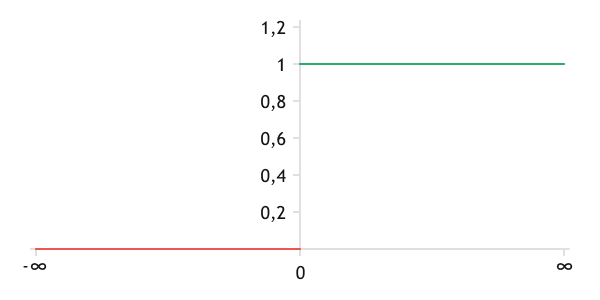
Threshold (step) activation function
This activation function is easy to understand, but its main drawback is the complexity or even the impossibility of training the neural network. The fact is that neural network training algorithms use the first-order derivative. However, the derivative of the function under consideration is always zero, except for x=θ (it is not defined at this point).
It is quite easy to implement this function in the form of MQL5 program code. The theta constant defines the level at which the neuron will be activated. When calling the activation function, we pass the pre-calculated weighted sum of the initial data in the parameters. Inside the function, we compare the value obtained in the parameters with theta activation level and return the activation value of the neuron.
const double theta = 0; |
The Python implementation is also quite straightforward.
theta = 0 |
Linear activation function
The linear activation function is defined by a linear function:
Where:
- a defines the angle of inclination of the line.
- b is the vertical displacement of the line.
As a special case of the linear activation function, if a=1 and b=0, the function has the form .
The function can generate values in the range from to and is differentiable. The derivative of the function is constant and equal to a, which facilitates the process of training the neural network. The mentioned properties allow for the widespread use of this activation function when solving regression problems.
It should be noted that computing the weighted sum of neuron inputs is a linear function. The application of a linear activation function gives a linear function of the entire neuron and neural network. This property prevents the use of the linear activation function for solving nonlinear problems.
At the same time, by creating nonlinearity in the hidden layers of the neural network by using other activation functions, we can use the linear activation function in the output layer neurons of our model. Such a technique can be used to solve nonlinear regression problems.
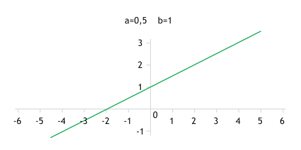
Graph of a linear function
The implementation of the linear activation function in the MQL5 program code requires the creation of two constants: a and b. Similarly to the implementation of the previous activation function, when calling the function, we will pass the pre-calculated weighted sum of inputs in the parameters. Inside the function, the implementation of the calculation part fits into one line.
const double a = 1.0; |
In Python, the implementation is similar.
a = 1.0 |
Logistic activation function (Sigmoid) #
The logistic activation function is probably the most common S-shaped function. The values of the function range from 0 to 1, and they are asymmetrical relative to the point [0, 0.5]. The graph of the function resembles a threshold function, but with a smooth transition between states.
The mathematical formula of the function is as follows:
This function allows the normalization of the output values of the function in the range [0, 1]. Due to this property, the use of the logistic function introduces the concept of probability into the practice of neural networks. This property is widely used in the output layer neurons when solving classification problems, where the number of output layer neurons equals the number of classes, and an object is assigned to a particular class based on the highest probability (maximum value of the output neuron).
The function is differentiable over the entire interval of permitted values. The value of the derivative can be easily calculated through the function value using the formula:
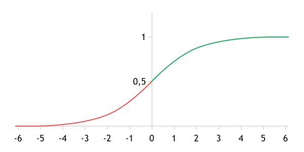
Graph of the logistic function (Sigmoid)
Sometimes a slightly modified logistic function can be used in neural networks:
Where:
- a stretches the range of function values from 0 to a.
- b, similarly to a linear function, shifts the resulting value.
The derivative of such a function is also calculated through the value of the function using the formula:
In practice, the most common applications are , so that the graph of the function is asymmetric with respect to the origin.
All of the above properties add to the popularity to using the logistic function as a neuron activation function.
However, this function also has its flaws. For input values less than −6 and greater than 6, the function value is pressed to the limits of the range of function values, and the derivative tends to zero. As a consequence, the error gradient also tends to zero. This leads to a decrease in the training rate of the neural network, and sometimes even makes the network nearly untrainable.
Below I propose to consider the implementation of the most general version of the logistic function with two constants a and b. Let's calculate the exponent using exp().
const double a = 1.0; |
When implementing in Python, before using the exponent function, you must import the math library, which contains the basic math functions. The rest of the algorithm and the function implementation are similar to the implementation in MQL5.
import math
|
Hyperbolic tangent (tanh) #
An alternative to the logistic activation function is the hyperbolic tangent (Tanh). Just like the logistic function, it has an S-shaped graph, and the function values are normalized. But they belong to the range from −1 to 1, and the the neuron state is changed out 2 times faster. The graph of the function is also asymmetric, but unlike the logistic function, the center of asymmetry is at the center of coordinates.
The function is differentiable on the entire interval of permitted values. The derivative value can be easily calculated through the function value using the formula:
The hyperbolic tangent function is an alternative to the logistic function, which quite often converges faster.
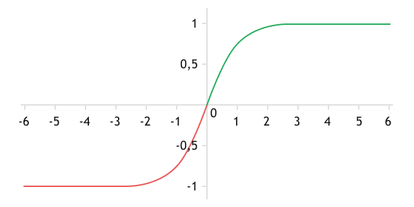
Graph of the hyperbolic tangent function (TANH)
But it also has the main drawback of the logistic function: during saturation of the function, when the function values approach the boundaries of the value range, the derivative of the function approaches zero. As a result, the gradient of the error tends to zero.
The hyperbolic tangent function is already implemented in the programming languages we use, and it can be called by simply calling the tanh() function.
double ActTanh(double x) |
The implementation in Python is similar.
import math
|
Rectified line unit (ReLU) #
Another widely used activation function for neurons is ReLU (rectified linear unit). When the input values are greater than zero, the function returns the same value, similar to a linear activation function. For values less than or equal to zero, the function always returns 0. Mathematically, this function is expressed by the following formula:
The graph of the function is something between a threshold function and a linear function.
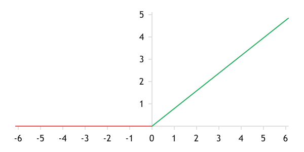
Graph of the ReLU function
ReLU, probably, is one of the most common activation functions at the moment. It has become so popular due to its properties:
- Like the threshold function, it operates based on the principle of a biological neuron, activating only after reaching a threshold value (0). Unlike the threshold function, when activated, the neuron returns a variable value rather than a constant.
- The range of values is from 0 to , which allows us to use the function in solving regression problems.
- When the function value is greater than zero, its derivative is equal to one.
- The function calculation does not require complex computations, which accelerates the training process.
The literature provides examples where neural networks with ReLU are trained up to 6 times faster than networks using TANH.
However, the use of ReLU also has its drawbacks. When the weighted sum of the inputs is less than zero, the derivative of the function is zero. In such a case, the neuron is not trained and does not transmit the error gradient to the preceding layers of the neural network. In the process of training there is a probability to get such a set of weights that the neuron will be deactivated during the whole training cycle. This effect has been called "dead neurons".
Subjectively, the presence of dead neurons can be detected by observing the increase in the learning rate: the more the learning rate accelerates with each iteration, the more dead neurons the network contains.
Several variations of this function have been proposed to minimize the effect of dead neurons when using ReLU, but they all boil down to one thing: applying a certain coefficient a for a weighted sum less than zero.
LReLU |
Leaky ReLU |
a = 0.01 |
PReLU |
Parametric ReLU |
The parameter a is selected in the process of training the neural network |
RReLU |
Randomized ReLU |
The parameter a is set randomly when the neural network is created |
The classical version of ReLU is conveniently realized using the max() function. Implementing its variations will require the creation of a constant or variable a. The initialization approach will depend on the chosen function (LReLU / PReLU / RReLU). Inside our activation function, we will create logical branching, depending on the value of the received parameter.
const double a = 0.01; |
In Python, the implementation is similar.
a = 0.01 |
Softmax #
While the previously mentioned functions were calculated solely for individual neurons, the Softmax function is applied to all neurons of a specific layer in a network, typically the last layer. Similar to sigmoid, this function uses the concept of probability in neural networks. The range of values of the function lies between 0 and 1, and the sum of all output values of neurons of the taken layer is equal to 1.
The mathematical formula of the function is as follows:
The function is differentiable over the entire interval of values, and its derivative can be easily calculated through the value of the function:
The function is widely used in the last layer of the neural network in classification tasks. The output value of the neuron normalized by the Softmax function is said to indicate the probability of assigning the object to the corresponding class of the classifier.
It is worth noting that Softmax is computationally intensive, which is why its application is justified in the last layer of neural networks used for multi-class classification.
The implementation of the Softmax function in MQL5 will be slightly more complicated than the examples discussed above. This is due to the processing of the neurons of the entire layer. Consequently, the function will receive a whole array of data in its parameters rather than a single value.
It should be noted that arrays in MQL5, unlike variables, are passed to function parameters by pointers to memory elements rather than by values.
Our function will take pointers to two data arrays X and Y as parameters and return a logical result at the end of the operations. The actual results of the operations will be in the array Y.
In the function body, we first check the size of the source data array X. The resulting array must be of non-zero length. We then resize the array to record the Y results. If any of the operations fails, we exit the function with the result false.
bool SoftMax(double& X[], double& Y[]) |
Next, we organize two loops. In the first one, we calculate exponents for each element of the obtained data set and summarize the obtained values.
//--- Calculation of exponent for each element of the array |
In the second loop, we normalize the values of the array created in the first loop. Before exiting the function, we return the obtained values.
//--- Normalization of data in an array |
In Python, the implementation looks much simpler since the Softmax function is already implemented in the Scipy library.
from scipy.special import softmax |
Swish #
In October 2017, a team of researchers from Google Brain worked on the automatic search for activation features. They presented the results in the article "Searching for Activation Functions". The article summarizes the results of testing a range of features against ReLU. The best performance was achieved in neural networks with the Swish activation feature. The replacing of ReLU with Swish (without retraining) improved the performance of the neural networks.
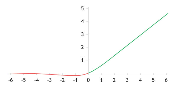
Graph of the Swish function
The mathematical formula of the function is as follows:
The parameter β affects the nonlinearity of the function and can be taken as a constant during network design, or can be selected during training. When β=0, the function reduces to a linearly scaled function.
When β=1, the graph of the Swish function approaches ReLU. But unlike the latter, the function is differentiable over the entire range of values.
A function is differentiable and its derivative is calculated through the value of the function. But unlike the sigmoid, it also requires an input value to calculate the derivative. The mathematical formula for the derivative is of the form:
The implementation of the function in the MQL5 program code is similar to the Sigmoid presented above. The parameter a is replaced by the obtained value of the weighted sum and the nonlinearity parameter β is added.
const double b=1.0; |
The implementation in Python is similar.
import math
|
It is worth noting that this is by no means a complete list of possible activation functions. There are different variations to the functions mentioned above, as well as different functions can be utilized altogether. Activation functions and threshold values should be selected by the architect of the neural network. It is not always the case that all neurons in a network have the same activation function. Neural networks in which the activation function varies from layer to layer are widely used in practice. Such networks are called heterogeneous networks.
Later we will see that, for implementing neural networks, it is much more convenient to utilize vector and matrix operations, which are provided in MQL5. This in particular concerns activation functions, because matrix and vector operations provide the Activation function which calculate activation functions for the whole data array with one line of code. In our case, the function would be calculated for the entire neural layer. The implementation of the function is as follows.
bool vector::Activation( |
In its parameters, the function receives a pointer to a vector or matrix (depending on the data source) for storing results, along with the type of activation function used. It should be noted that the range of activation functions in MQL5 vector/matrix operations is much wider than described above. Their complete list is given in the table.
Identifier |
Description |
|---|---|
AF_ELU |
Exponential linear unit |
AF_EXP |
Exponential |
AF_GELU |
Linear unit of Gauss error |
AF_HARD_SIGMOID |
Rigid sigmoid |
AF_LINEAR |
Linear |
AF_LRELU |
Leaky linear rectifier (Leaky ReLU) |
AF_RELU |
Truncated linear transformation ReLU |
AF_SELU |
Scaled exponential linear function (Scaled ELU) |
AF_SIGMOID |
Sigmoid |
AF_SOFTMAX |
Softmax |
AF_SOFTPLUS |
Softplus |
AF_SOFTSIGN |
Softsign |
AF_SWISH |
Swish function |
AF_TANH |
Hyperbolic tangent |
AF_TRELU |
Linear rectifier with threshold |