Multilayer perceptron and backpropagation algorithm

Introduction

• The popularity of these two methods grows, so a lot of libraries have been developed in Matlab, R, Python, C++ and others, which receive a training set as input and automatically create an appropriate network for the problem.

• However, when using ready-made libraries, it can be difficult to understand what exactly is happening and how we get an optimized network. The understanding of solution basics is essential for further development of these methods. In this article, we will create a very simple structure of a neural network architecture.

• Let us try to understand how the basic neural network type works (including single-neuron perceptron and multilayer perceptron). We will consider an exciting algorithm which is responsible for network training (gradient descent and backpropagation). Existing complex models are often based on such simple network models.

A brief overview of history

• The first neural network was proposed by Warren McCulloch and Walter Pitts in 1943. They wrote a great article on how neurons should work. They also built a model based on their ideas: they created a simple neural network with electrical circuits.

• Artificial intelligence research progressed rapidly, and in 1980, Kunihiko Fukushima developed the first real multilayered neural network.

• The original purpose of a neural network was to create a computer system capable of solving problems in a way similar to the human brain. However, as time went by, the researchers changed their focus and started using neural networks to solve various specific tasks. Now, neural networks perform a wide variety of tasks, including computer vision, voice recognition, machine translation, social media filtering, board games or video games, medical diagnostics, weather forecasting, time series forecasting, images/text/voice recognition, and more.

Computer model of neuron: perceptron

Perceptron

The perceptron was inspired by the idea of processing information from a single nerve cell called a neuron. A neuron receives signals as input through its dendrites, which transmit an electrical signal to the cell body. Similarly, the perceptron receives input signals from training data sets, which have been previously weighted and combined into a linear equation called activation.

• z = sum(weight_i * x_i) + bias

Here 'weight' is the network weight, 'X' is an input, 'i' is the index of a weight or input, and bias is a special weight which has no multiplier input (thus we can assume that input is always 1.0).

Then the activation is transformed into an output (forecast) value using a transfer function (activation function).

• y = 1.0 if z >= 0.0, otherwise 0.0

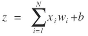
Thus, the perceptron is a two-class problem classification algorithm (binary classifier), where a linear equation can be used to separate the two classes.

This is closely related to Linear Regression and Logistic Regression, which generate predictions in a similar way (for example, as a weighted sum of inputs).

The perceptron algorithm is the simplest artificial neural network type. It is a single-neuron model which can be used for two-class classification problems. It also provides the basis for the further development of considerably larger networks.

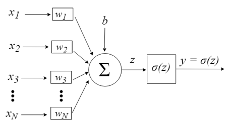
Neuron inputs are represented by the vector x = [x1, x2, x3,…, xN], which can correspond, for example, to an asset price series, technical indicator values or image pixels. When they reach the neuron, they are multiplied by appropriate synaptic weights - the elements of the vector w = [w1, w2, w3, ..., wN]. This generates the z value( commonly referred to as "Activation Potential") by the following formula:

b provides a higher degree of freedom and it for not depend on the input. Usually this corresponds to the a "bias". The z value then passes through the σ activation function, which is responsible for limiting this value in a certain interval (for example, 0 - 1), which produces the final output and the neuron value. Some of the used activation functions include step, sigmoid, hyperbolic tangent, softmax and ReLU ("rectified linear unit").

Let us view the process aimed at reaching the class separability limit, using two situations demonstrating their convergence towards stabilization, considering only two inputs {x1 and x2}

The weights of the perceptron algorithm should be estimated based on training data using stochastic gradient descent.

Stochastic gradient

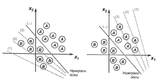
Gradient descent is the process of minimizing a function in the direction of the gradients of the cost function.

This implies knowing the cost form, as well as the derivative, so that we can know the gradient from a certain point and can move in this direction, for example, downwards, towards the minimum value.

In machine learning, we can use a technique that evaluates and updates the weights for each iteration, called Stochastic Gradient Descent. Its purpose is to minimize a model error in our training data.

The idea of this algorithm is that each training instance is shown to the model one at a time. The model creates a forecast for the training instance. Then an error is calculated and the model is updated to reduce the error in the next forecast.

This procedure can be used to find a set of model weights which produce the lowest error.

For the Perceptron algorithm, weights w are updated at each iteration, using the following equation:

• w = w + learning_rate * (expected - predicted) * x

Where w is an optimizable value, learning_rate is a learning rate that you should set (for example, 0.1), (expected - predicted) is the forecast error for a model regarding the weight, and x is an input.

The Stochastic Gradient Descent requires two parameters:

• Learning rate: used to limit by how much each weight is corrected during each update.
• Epochs - how many times to run through training data when updating the weight.

These, along with the training data, will be the arguments for the function.

We need to execute 3 loops in the function:

1. Loop for each epoch.

2. Loop for each line in the training data for an epoch.

3. Loop for each weight, in which one line is updated in a time.

Weights are updated based on the error made by the model. An error is calculated as a difference between the actual value and the forecast made using the weights.

Each input attribute has its own weight. The weights are constantly updated, for example:

• w(t+1)= w(t) + learning_rate * (expected(t) - predicted(t)) * x(t)

The bias is updated in a similar way, except for the input, because there is no specific input for a bias:

• bias(t+1) = bias(t) + learning_rate * (expected(t) - predicted(t)).

Applying the neuron model

Now, let's move on to practical application.

This section is divided into two parts:

1. Making predictions

2. Optimizing the network weight

These steps provide a basis for implementing and applying the perceptron algorithm to other classification problems.

We need to define the number of columns in the set X. For this, we need to define a constant

#define nINPUT 3

---

In MQL5, a multidimensional array can be static or dynamic only for the first dimension. Therefore, since all other dimensions will be static, size must be specified during array declaration.

 

1. Making predictions

The first step is to develop a function that can make predictions.

This will be necessary both when evaluating the weights of candidates during stochastic gradient descent, and after the completion of the model. Prediction should be made based on test data and based on new data.

Below is the predict function, which forecasts the output value based on a specific set of weights.

The first weight is always a bias because it is autonomous, so it does not work with a specific input value.

// Make a prediction with weights
template <typename Array>
double predict(const Array &X[][nINPUT], const Array &weights[], const int row=0)
  {
   double z = weights[0];
   for(int i=0; i<ArrayRange(X, 1)-1; i++)
     {
      z+=weights[i+1]*X[row][i];
     }
   return activation(z);
  }

Neuron transfer:

Once a neuron is activated, we need to transfer the activation to view the actual outputs of the neuron.

//+------------------------------------------------------------------+
//|                Transfer neuron activation                        |
//+------------------------------------------------------------------+
double activation(const double activation) //#
  {
   return activation>=0.0?1.0:0.0;
  }

We input into the prediction function the input set X, an array of weights (W) and the line for which the input set X is predicted.

Let us use a small data set to check the prediction function.

We can also use pre-prepared weights for making predictions for this dataset.

double weights[] = {-0.1, 0.20653640140000007, -0.23418117710000003};

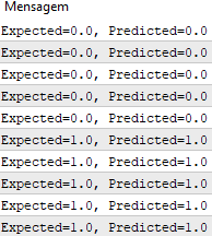
After putting it all together, we can test the forecast function.

#define nINPUT 3
//+------------------------------------------------------------------+
//| Script program start function                                    |
//+------------------------------------------------------------------+
void OnStart()
  {
//---
   random.seed(42);
   double dataset[][nINPUT] = {     //X1     //X2   //Y  
                               {2.7810836,2.550537003,0},
                               {1.465489372,2.362125076,0},
                               {3.396561688,4.400293529,0},
                               {1.38807019,1.850220317,0},
                               {3.06407232,3.005305973,0},
                               {7.627531214,2.759262235,1},
                               {5.332441248,2.088626775,1},
                               {6.922596716,1.77106367,1},
                               {8.675418651,-0.242068655,1},
                               {7.673756466,3.508563011,1}
                              };
   double weights[] = {-0.1, 0.20653640140000007, -0.23418117710000003};
   for(int row=0; row<ArrayRange(dataset, 0); row++)
     {
      double predict = predict(dataset, weights, row);
      printf("Expected=%.1f, Predicted=%.1f", dataset[row][nINPUT-1], predict);
     }
  }
//+------------------------------------------------------------------+
// Make a prediction with weights
template <typename Array>
double predict(const Array &X[][nINPUT], const Array &weights[], const int row=0)
  {
   double z = weights[0];
   for(int i=0; i<ArrayRange(X, 1)-1; i++)
     {
      z+=weights[i+1]*X[row][i];
     }
   return activation(z);
  }
//+------------------------------------------------------------------+
//|                Transfer neuron activation                        |
//+------------------------------------------------------------------+
double activation(const double activation) //#
  {
   return activation>=0.0?1.0:0.0;
  }

There are two input values (X1 and X2)and three weights (bias, w1 and w2). The activation equation for this problem looks as follows:

activation = (w1 * X1) + (w2 * X2) + b

Or with specific weights, it is manually set as:

activation = (0.206 * X1) + (-0.234 * X2) + -0.1

After the function execution, we get predictions that correspond to the expected output values y.

We can now implement stochastic gradient descent to optimize the weight values.

2. Optimizing network weights

As mentioned earlier, weights for training data can be evaluated using stochastic gradient descent.

Below is the train_weights() function which calculates weights for a training data set, using stochastic gradient descent.

There is no way to return a result from this training data set array in MQL5, as, unlike variables, arrays can only be passed to a function by reference. This means that the function does not create its own instance of the array. Instead, it works directly with the array passed to it. Thus, all changes made to that array within the function affect the original array.

 //+------------------------------------------------------------------+
//|  Estimate Perceptron weights using stochastic gradient descent   |
//+------------------------------------------------------------------+
template <typename Array>
void train_weights(Array &weights[], const Array &X[][nINPUT], double l_rate=0.1, int n_epoch=5)
  {
   ArrayResize(weights, ArrayRange(X, 1));
   for(int i=0; i<ArrayRange(X, 1); i++)
     {
      weights[i]=random.random();
     }
     
   for(int epoch=0; epoch<n_epoch; epoch++)
     {
      double sum_error = 0.0;
      for(int row=0; row<ArrayRange(X, 0); row++)
        {
         double y = predict(X, weights, row);
         double error = X[row][nINPUT-1] - y;
         sum_error += pow(error, 2);
         weights[0] = weights[0] + l_rate * error;

         for(int i=0; i<ArrayRange(X, 1)-1; i++)
           {
            weights[i+1] = weights[i+1] + l_rate * error * X[row][i];
           }
        }
      printf(">epoch=%d, lrate=%.3f, error=%.3f",epoch, l_rate, sum_error);
     }
  }

In each epoch, we track the sum of squared error (positive value) to monitor the decrease in error. So we can view how the algorithm moves towards error minimization from epoch to epoch.

We can test our function with the same data set presented above.

#define nINPUT 3
//+------------------------------------------------------------------+
//| Script program start function                                    |
//+------------------------------------------------------------------+
void OnStart()
  {
//---
   random.seed(42);
   double dataset[][nINPUT] = {     //X1     //X2   //Y  
                               {2.7810836,2.550537003,0},
                               {1.465489372,2.362125076,0},
                               {3.396561688,4.400293529,0},
                               {1.38807019,1.850220317,0},
                               {3.06407232,3.005305973,0},
                               {7.627531214,2.759262235,1},
                               {5.332441248,2.088626775,1},
                               {6.922596716,1.77106367,1},
                               {8.675418651,-0.242068655,1},
                               {7.673756466,3.508563011,1}
                              };
   double weights[];
   train_weights(weights, dataset);
   ArrayPrint(weights, 20);
   for(int row=0; row<ArrayRange(dataset, 0); row++)
     {
      double predict = predict(dataset, weights, row);
      printf("Expected=%.1f, Predicted=%.1f", dataset[row][nINPUT-1], predict);
     }
  }
//+------------------------------------------------------------------+
// Make a prediction with weights
template <typename Array>
double predict(const Array &X[][nINPUT], const Array &weights[], const int row=0)
  {
   double z = weights[0];
   for(int i=0; i<ArrayRange(X, 1)-1; i++)
     {
      z+=weights[i+1]*X[row][i];
     }
   return activation(z);
  }
//+------------------------------------------------------------------+
//|                Transfer neuron activation                        |
//+------------------------------------------------------------------+
double activation(const double activation) //#
  {
   return activation>=0.0?1.0:0.0;
  }
//+------------------------------------------------------------------+
//|  Estimate Perceptron weights using stochastic gradient descent   |
//+------------------------------------------------------------------+
template <typename Array>
void train_weights(Array &weights[], const Array &X[][nINPUT], double l_rate=0.1, int n_epoch=5)
  {
   ArrayResize(weights, ArrayRange(X, 1));
   ArrayInitialize(weights, 0);
     
   for(int epoch=0; epoch<n_epoch; epoch++)
     {
      double sum_error = 0.0;
      for(int row=0; row<ArrayRange(X, 0); row++)
        {
         double y = predict(X, weights, row);
         double error = X[row][nINPUT-1] - y;
         sum_error += pow(error, 2);
         weights[0] = weights[0] + l_rate * error;

         for(int i=0; i<ArrayRange(X, 1)-1; i++)
           {
            weights[i+1] = weights[i+1] + l_rate * error * X[row][i];
           }
        }
      printf(">epoch=%d, lrate=%.3f, error=%.3f",epoch, l_rate, sum_error);
     }
  }

Learning rate is 0.1, the model is trade only for 5 epochs for the entire data set.

During execution, a message with the squared error sum is printed for each epoch, as well as the final data set.

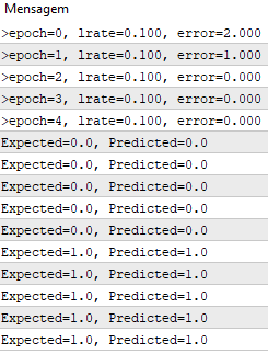
We see how quickly the algorithm has learned the problem.

This test is available in the PerceptronScript.mq5 file attached below.

Multilayer Perceptron

• Combining neurons into layers

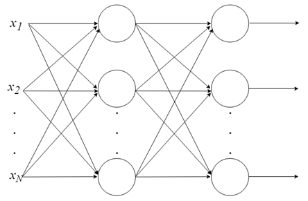
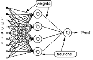
   There is not much that can be done with a single neuron. But neurons can be combined into a multilayer structure, each layer having a different number of neurons, and form a neural network called a Multi-Layer Perceptron, MLP. The input vector X passes through the initial layer. The output values of this layer are input into the next and so on, until the last layer outputs the final result. The network can be organized in several layers, making it deep and capable of learning increasingly complex relationships.

MLP training

   Before a network starts working, this network needs to be trained. It is like teaching a child to read. Supervised training is used to train the MLP in the context of machine learning, but how does it work?

Supervised Learning:

• We have a set of labeled data, and we already know which is the correct output. The learning is based on the idea that there is a connection between the input and the output.
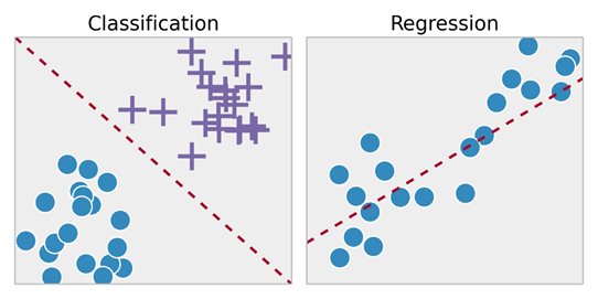
• Supervised learning problems are subdivided into "regression" and "classification" problems. In regression problems, we try to predict the results on a continuous output, which means that we try to map input variables to some continuous function. In classification problems, we try to predict the results in a discrete output. In other words, we try to map the input variables into different categories.

Example 1:

• Based on a dataset of house sizes in the real estate market, try to predict their price. Price depending on the size is a continuous result, so this is a regression problem.
• This problem could be turned into a classification problem - to predict whether "the house can be sold for more or less that the specified price". Here the houses will be grouped by price into two different categories.

Backpropagation

Undoubtedly Backpropagation is the most important algorithm in the history of neural networks. Without efficient backpropagation, it would be impossible to train deep learning networks the way we do today. Backpropagation can be considered the cornerstone of modern neural networks and deep learning.

Aren't we learning from mistakes?

The idea behind the backpropagation algorithm is as follows: based on the calculation error that occurred in the output layer of the neural network, recalculate the W vector weight weights of the last layer of neurons. Then move to the previous layers, from back to front. So, the algorithm implies the updating of W weights of all layers, from the last one to the input layer of the network, by backpropagating the error received by the network. In other words, it calculates an error between what the network predicted and what it actually was (actual 1, predicted 0; we have an error!), so recalculate the values of all weights, starting with the last layer and going to the first, always paying attention to how this error is reduced.

The backpropagation algorithm consists of two steps:

1. Forward Pass: inputs pass through the network and receive output predictions (this step is also known as the propagation step).

2. Backward Pass: the loss function gradient is calculated in the network's final layer (prediction layer). It is used then for recursive application of the chain rule to update the weights in our network (also known as weight update or backpropagation)

Consider the network with a layer of hidden neurons and an output neuron. When the input vector propagates over the network, there is an output Pred(y) for the current set of weights. The purpose of supervised training is to adjust the weights in order to reduce the difference between Pred(y) and the required output Req(y). This requires an algorithm that reduces the absolute error, which is similar to reducing the squared error, where:

(1)

Network error = Pred - Req

      = E

 

The algorithm should adjust weights aiming to minimize E². Backpropagation is an algorithm that minimizes the E² by gradient descent. To minimize E², it is necessary to calculate its sensitivity to each weight. In other words, we need to know the effect of a change in each weight on E². If we know this effect, we will be able to adjust the weight towards a decrease in the absolute error. The below diagram shows how the backpropagation rule works.

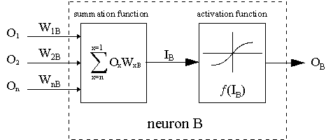
The dotted line indicates neuron B, which can be a hidden or output neuron. The outputs of n neurons (O 1 ... O n) at the previous layer serve as input data for the neuron B. If neuron B is in the hidden layer, it is simply an input vector. The outputs are multiplied by the appropriate weights (W1B ... WnB), where WnB is the weight connecting neuron n and neuron B. The sum function adds all of these products to get the input IB, which is processed by the trigger function f(.) of neuron B. f (IB) is the output OB of neuron B. To illustrate this, let us neuron 1 be called A and consider the weight WAB connecting the two neurons. The approach to updating the weight is based on the delta rule:

(2)

where - is the learning rate parameter, and

is the sensitivity of error E² to the weight WAB; it determines the search direction in the weight space for the new WAB weight, as shown in figure below.

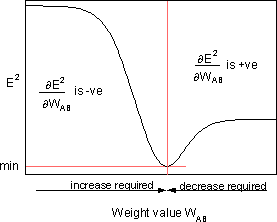
To minimize E², the delta rule provides the required weight change direction.

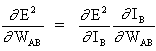
The key concept of the above equation is to evaluate the expression ∂E² /∂WAB, which consists in calculating partial derivatives of the E² error function, with respect to each weight of the vector W.

Chain Rule:

(3)

and

(4)

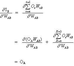
since other neuron inputs do not depend on weight WAB. Thus, based on equations (3) and (4), equation (2) becomes

(5)

and WAB weight change depends on the sensitivity of the squared error E² at the input IB, on the unit of B and the input signal OА.

Two situations are possible:

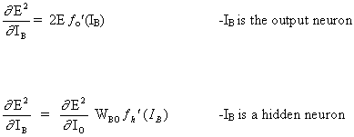
1. B is an output neuron;

2. B is a hidden neuron.

Consider the first case:

Since B is an output neuron, a change in the squared error due to the adjustment of WAB is simply a change in the squared error of the output signal B.

(6)

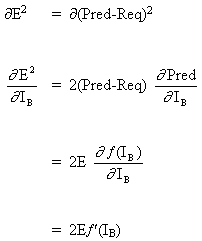
combine equations (5) and (6), to obtain

(7)

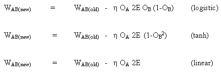
The rule for changing weights, when neuron B is an output neuron, if the output activation function f (.) is a logistic function:

(8)

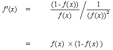
Differentiate equation (8) with respect to the argument x:

(9)

But

(10)

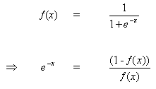
when inserting (10) to (9), we get:

(11)

the same way for function tanh

or for the linear function (identity)

Thus, we get:

Consider the second case

B is a hidden neuron

(12)

where O is the output neuron

(13)

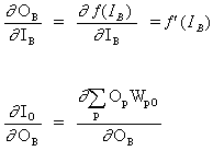
where p is an index covering all neurons, including neuron B, which provides input signals to the output neuron. Expand the right pert of equation (13),

(14)

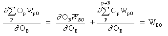
since weights of other neurons WpO (p! = B) do have no dependence on OB.

When inserting (13) and (14) to (12):

(15)

Consequently, is now expressed as a function of , calculated as is described in equation (6).

The full rule for updating the weight WAB between neuron A which sends a signal to neuron B, is as follows:

(16)

where

where fo (.) and fh (.) are hidden activation and output functions, respectively.

Example

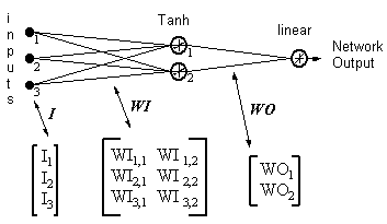
Network output = [tanh(I ^T .WI)] . WO

HID = [Tanh(I ^T.WI)] ^T- outputs of hidden neurons

ERROR = (network output - required output)

LR = Learning Rate

Weight updates become,

 

linear output neuron:

(17)

WO = WO - ( LR x ERROR x HID )

hidden neuron:

(18)

WI = WI - { LR x [ERROR x WO x (1- HID ²)] . I ^T } ^T

 

Equations 17 and 18 show that the weight update is an input multiplied by the local gradient. This provides the direction, the magnitude of which also depends on the magnitude of the error. If we take a direction without magnitude, all changes will be the same size, and this will depend on the learning rate. The above algorithm is a simplified version since there is only one output neuron. The original algorithm can have more than one output, while a decrease in the gradient minimizes the total squared error of all outputs. There are many other algorithms that evolved from the original algorithm in an effort to increase the learning rate. They are summarized in:

 

"Back Propagation family album" - Technical report C/TR96-05, Department of Computing, Macquarie University, NSW, Australia.

 

Backpropagation is an elegant and ingenious algorithm. Modern deep learning models such as Convolutional Neural Networks, which have shown much superior performance in tasks related to image classification, or Recurrent Neural Networks, which are used for Natural Language Processing tasks, also use the back propagation algorithm. The most incredible thing is that such models can find patterns which cannot be observed and understood by humans. It is really fascinating, and it allows us to expect further development of deep learning algorithms, which will help us solve many of the basic problems faced by humanity.

Application of the MLP model

This tutorial is divided into 5 parts:

1.       Network initialization.

2.       FeedForward.

3.       Backpropagation.

4.       Network training.

5.       Prediction.

 

Let us create an implementation in pure MQL. We already talked about libraries in other languages, which are much more complex. So, it is highly recommended to use these libraries for practical and performance reasons. However, it is important to understand the internals of such libraries in order to have more control over the whole process. No OOP is used in the below test, because it is only an algorithm demonstrating the earlier discussed equations, so OOP is not really necessary here. However, please note that in real-life cases it is much more practical to use OOP, since it provides the scalability of the project.

1. Network initialization

Each neuron has a set of weights that need to be maintained, weight for each input connection and additional weight for bias.

It is recommended to initialize network weights for small random numbers. In this case, random numbers ranging from 0 to 1 will be used. For this purpose, we have created a function generating random numbers.

double random(void)
  {
   return ((double)rand())/(double)SHORT_MAX;
  }

Below is the initialize_network() function which creates weights for our neural network.

// Forward propagate input to a network output
void forward_propagate(void)
  {
//calculate the outputs of the hidden neurons
//the hidden neurons are tanh
   int i = 0;
   for(i = 0; i<numHidden; i++)
     {
      hiddenVal[i] = 0.0;
      for(int j = 0; j<numInputs; j++)
        {
         hiddenVal[i] += (X[patNum][j] * weightsIH[j][i]);
        }
      hiddenVal[i] = tanh(hiddenVal[i]);
     }
//calculate the output of the network
//the output neuron is linear
   outPred = 0.0;
   for(i = 0; i<numHidden; i++)
     {
      outPred += hiddenVal[i] * weightsHO[i];
     }
//calculate the error
   errThisPat = outPred - y[patNum];
  }

3. Backpropagation

The backpropagation algorithm is named in accordance with the way weights are trained

An error is calculated between the expected outputs and the feedforward network outputs. These errors are then propagated back through the network, from the output layer to the hidden layer, shifting responsibility for the error and updating the weights as they come in.

The math behind the backpropagation error mechanism has been explained above.

//+------------------------------------------------------------------+
//|        Backpropagate error and change network weights            |
//+------------------------------------------------------------------+
void backward_propagate_error(void)
  {
//adjust the weights hidden-output
   for(int k = 0; k<numHidden; k++)
     {
      double weightChange = LR_HO * errThisPat * hiddenVal[k];
      weightsHO[k] -= weightChange;
      //regularisation on the output weights
      regularisationWeights(weightsHO[k]);
     }
// adjust the weights input-hidden
   for(int i = 0; i<numHidden; i++)
     {
      for(int k = 0; k<numInputs; k++)
        {
         double x = 1 - pow(hiddenVal[i],2);
         x = x * weightsHO[i] * errThisPat * LR_IH;
         x = x * X[patNum][k];
         double weightChange = x;
         weightsIH[k][i] -= weightChange;
        }
     }
  }

The regularizationWeights method has been created only to regularize weights in the range between -5 and 5.

//regularisation on the output weights
void regularisationWeights(double &weight)
  {
   weight<-5?weight=-5:weight>5?weight=5:weight=weight;
  }

4. Network training

The network is trained using stochastic gradient descent.

This includes several iterations during which data is fed into the network, input is fed forward for each data line, error is propagated back, and weights are updated.

//# Train a network for a fixed number of epochs
void train(void)
  {
   for(int j = 0; j <= numEpochs; j++)
     {
      for(int i = 0; i<numPatterns; i++)
        {
         //select a pattern at random
         patNum = rand()%numPatterns;
         //calculate the current network output
         //and error for this pattern
         forward_propagate();
         backward_propagate_error();
        }
      //display the overall network error
      //after each epoch
      calcOverallError();
      printf("epoch = %d RMS Error = %f",j,RMSerror);
     }
  }

5. Prediction

Making predictions using a trained neural network is pretty straightforward.

We have already seen how to propagate the input pattern to receive the output. This is all we need to do in order to make a prediction. We can use the output values directly, as the probability that the pattern belongs to each output class.

// # Make a prediction with a network
void predict(void)
  {
   for(int i = 0; i<numPatterns; i++)
     {
      patNum = i;
      forward_propagate();
      printf("real = %d predict = %f",y[patNum],outPred);
     }
  }

A complete example is available in the MLP_Script.mq5 file attached below.

Conclusion

We have considered computations which are performed in the perceptron neuron development process, as well as a network of perceptron neurons called "Multilayer perceptron, MLP". We have also seen how this type of neural networks is trained using the backpropagation and gradient descent algorithms.