Brute force approach to pattern search (Part II): Immersion

Introduction

I decided to continue the topic which we started in the previous article. This time we will conduct an in-depth analysis of currency pairs using the modified application version. I would like to thank the user Aleksey Vyazmikin for his contribution to the project development. His advice was very useful in technical terms and pushed further development. I will continue this work in the next article and will provide more interesting data and results. I believe that it is very important to show the effectiveness of the analysis of a particular currency pair on a global scale, as well as to demonstrate the difference in the analysis of time intervals of maximum and minimum duration. Because my time and computing resources are limited, I was able to cover only a few currency pairs with only one timeframe. However, this seems to be enough for the first acquaintance with global patterns. When analyzing the data, I will additionally use the data from the previous article.

Why is this topic so interesting?

Very often all ideas for the MetaTrader 4 and MetaTrader 5 Expert Advisor programmers imply countless lines of code, countless tests, optimizations, back and forward tests. In most cases, we get not what we want. Some programmers get bored with this specific. The process of research and search turns into a routine. If the work does not bring any moral satisfaction and money, then you are very likely to quit. This is what happened to me. I decided to say goodbye to the routine and to start automating the actions that can be successfully performed by a machine. The machine has no emotions and it is an ideal worker, unlike me. Of course, the machine does not have such wide thinking as a person, but it has a lot of computing resources and can implement some processes easier and faster. I had a choice, to start writing my own neural network architecture capable of evolving, or to start with the simplest approach to solving the problem. I decided to use the latter approach. Despite its simplicity, the project gives room for creativity and interest, in contrast to simple programming of MQL products. It is a good idea to work on a universal template and to further develop it by gradually adding the necessary functionality. We can start with a simple template, and then create new templates for a specific operating principle. Thus, we can get rid of the boring routine and move on in our development. Well, laziness is the father of progress.

New Version of the Brute Force Program and a List of Changes

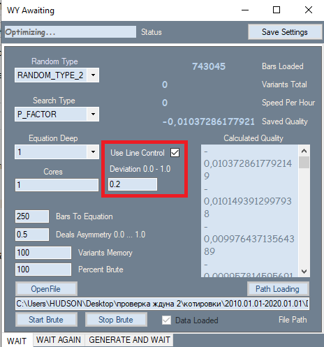
There was only one change in the program, which is shown in a red frame. This setting is taken from the second tab, where it has shown its best. The reason for adding this setting is that it has a very strong impact on the quality of the final results. During analysis, on the first tab, all results were initially sorted by quality. The profit factor or expected payoff in points was used as a quality criterion. But the program did not allow us the evaluation of the graph shape. I used the linearity factor (similarity to a straight line) as a shape criterion, which saves us from the need to visually check each option. Here we can come to the conclusion that straighter and smoother graphs are more likely to give a high-quality variant on the second tab. Also such graphs have a reduced number of variants that will be discarded by a filter on the second tab. A second pass is required for calculating this value. If this filter is active, the brute force speed is about 2 times slower. But it is not the speed that is important to us, but the total number of primary results obtained, as their quality affects further performance.

In addition to the introduced filter, the polynomial itself has changed. Now the polynomial accepts not only Close[i]-Open[i] values of specific bars as arguments, but also the following values:

• Close[i]-Open[i]
• High[i]-Open[i]
• Low[i]-Close[i]
• Low[i]-Open[i]
• High[i]-Close[i]

Now the formula includes all price data of a specific bar, unlike the previous version of the program. This greatly increases the complexity of the polynomial, which leads to a decrease in the brute force speed. But now we can select better and more efficient market formulas, provided there are enough computing resources. Of course, we could create other variables with these data. But when these values are used in the polynomial, you obtain those values that can be a linear combination of the above values, for example: 

• C1*(High[i]-Close[i]) + C2*(Low[i]-Close[i]) = NewQuant
• if  C1 = 1 and C2 = -1
• NewQuant = (High[i]-Close[i]) - (Low[i]-Close[i]) =  High[i]-Low[i]
• in other cases
• NewQuant = (C1-C3)*(High[i]-Close[i])+(C2+C3)*(Low[i]-Close[i])  +  C3*((High[i]-Close[i]) - (Low[i]-Close[i])) = (C1-C3)*(High[i]-Close[i])+(C2-C3)*(Low[i]-Close[i]) +  C3*(High[i]-Low[i])

In other words, using a linear combination of variables, which in turn consist of linear combinations of other variables, we can compose new variables without even including them in the basic formula. It is better to try not to include those variables that can be formed from others which are already present in the formula. They will appear during the selection of coefficients, depending on the values of the coefficients themselves.

As a result, the new polynomial will be much more complicated:

• Y = Sum(0,NC-1)( C[i]*Variant of product(x[1]^p[1]*x[2]^p[2]...*x[N]^p[N]) )
  
• Sum(0,N)(p[i])=MaxPowOfPolinom
• NC - the total number of terms in the polynomial, which is equal to the number of selected coefficients
  

where x[i] are arguments that the polynomial takes, and p[i] is the degree to which the argument is raised. The total degree of all constituent factors should not exceed the allowed number for our polynomial, because no computer can handle such complex expansions. I almost always use degree 1 or 2 or 3, when the number of bars for the formula is minimal. Anyway, the use of higher degrees is ineffective, even on the servers. There is not enough computing power.

Below are the argument options. The final sum includes all possible combinations of products:

1. x[i] =Close[i]-Open[i]
2. x[i] =High[i]-Open[i]
3. x[i] =Low[i]-Close[i]
4. x[i] =High[i]-Open[i]
5. x[i] =High[i]-Close[i]

I would also like to clarify why we perform all these actions with the polynomial. The point is that any system ultimately comes down to a set of conditions. There can be one or several conditions, which doesn't matter, because conditions are a logical function. A set of conditions can ultimately be converted to a boolean expression that returns either true or false. Such a signal can only interpreted as Yes or No. But it is impossible to determine how strong the signal is or to adjust the signal. If you use several indicators as signals, you can separately adjust the parameters of these indicators, which will lead to a change in the final logical expression or to a change in the signal, which will eventually affect trading. But I think that this is extremely inconvenient, because by changing one or another parameter of a particular indicator, we will not know how this will affect trading.

The main idea behind this approach was simplicity and efficiency. Why exactly this approach? It has several advantages:

• Uniqueness of the optimized function
• Dependence of the signal strength on the function value
• Ease of use
• The only optimizable parameter is the polynomial value

The most important thing is that we do not need to select the number of conditions and their type. This is because we originally accept the idea that instead of looking for an infinite set of conditions, we can reduce all these conditions to a single function which outputs either a positive fractional or negative fractional number. Depending on the reliability of one or another function, it may require a stronger signal in modulus. In some formulas this may provide scalability. Scalability here means the ability to amplify a signal when the number of deals decreases.

Generally speaking, my research, as those of many other people, leads to one single conclusion. An attempt to strengthen the entry signal inevitably leads to a decrease in the number of deals in a fixed period of time. In other words, for any function having a random component, some points always have a more predictable outcome than other points. If our function is efficient enough, then it can achieve certain predictability level with increasing requirements for the signal provided by this function. Of course, this is true not for every function which satisfies our primary conditions. But the stricter the primary conditions, the higher the expected payoff of those formula variants which we can find by using the brute force approach. This is also true for gradient boosting, as well as for other pattern search methods, including neural networks.

Much depends on the data sample. The smaller the sample, the greater the chance of getting a random result. A random result here is a result that either does not work, or works extremely ineffectively when testing the final system on the global history of the symbol on which the pattern was searched.

We will try to answer the question of how the future quality of the final trading system depends on the size of the analyzed data area and the amount of labor required to find this system. First, let us define the formula for the mathematical expectation of the number of found strategies over a fixed period of time:

• Mn(t) = W(t,F)*Ef(T,N,L)
• Mn -  mathematically expected number of found strategies which meet the our requirements
• W(t,F) = F*t - the resulting number of checked variants per unit of time
• Ef(T,N,L) = ? - brute force efficiency, which depends on the interval length, quote type, the required number of closed orders and the required linearity factor if it is taken into account during brute force (this value is equal to the probability that the results of the current variant will take the necessary and sufficient values)
  
• N - the minimum allowable number of deals which would be enough for our test
• L - the maximum allowable linearity factor (as an additional control criterion)
• F - strategy variants brute force frequency

It is extremely difficult to determine the form of the Ef function, but we can roughly estimate how it will look and what properties it has:

In order to be able to show a multidimensional function on a plane, it is necessary to fix all its arguments with some numbers, except for one argument, by which the graph itself is built. Especially interesting is the T variable, which denotes the duration of the analyzed sample in time, provided we analyze one timeframe. If we discard this assumption, then we can take the sample size as T - this will not change the graph appearance. Naturally, we are interested in how the remaining 2 arguments will affect the graph appearance. This is shown in the figure. The more orders we want to have in the final version, the fewer systems we will find that meet our requirements, simply because it is much easier to find a system with fewer orders. The same is true for the linearity factor (deviation from a straight line), however here the better linearity factor is the smaller one (tends to zero).

If we do not fix the concept of the system quality (because this value can be both a profit factor and a math expectation), then we can also introduce the concept of the maximum quality of the found system. We can similarly describe what it depends on:

• Mq=Mq(T,N,S)
• S - the selected formula configuration

In other words, the highest possible quality of the strategy directly depends on the effectiveness of our formula, as well as on our requirements and the complexity of the interval. At the same time, we still assume that the beginning of the area is fixed, and each variation of the training start point is unique and gives unique starting parameters. In other words, by choosing a different starting date for the training area, we will get different efficiency value and other parameters, as well as the final quality of the systems obtained.

We can also come to the understanding that each type of quality has its maximum value, for example, the profit factor's max quality is infinity, but I do not like to use this measure for analysis, because its max value is not limited, and thus graphical models with the PF will be harder to understand. Therefore, I use P_FACTOR, my own analogue of PF. It lies in the range [-1,1].

• P_FACTOR=(Profit-Loss)/(Profit+Loss)

Its maximum is equal to 1, and thus it is more convenient to work with. Here is the unction that describes the maximum of this value depending on T (selected area and its sample).

• Mx=Mx(T)

If the parameter or the quality criterion is P_FACTOR, then Mx(T)=1. The function form can be unknown, but it is known that Mx'(T) > 0 throughout the entire positive part of the T axis. It means that the value is positive at any point, and thus the chart is increasing all the time.

This will look as follows for the profit factor:

This example has an upper limit of the PF and two graphs showing two different formulas with different requirements. On the graph, the formula with the lime color is better, because it is less prone to quality fading as "T" tends to infinity.

This will look as follows for the mathematical expectation:

Here again we have two variants for two different formulas with different requirements. Additionally we have here Mx(T) which serves as an asymptote - Mq(T,N,S) cannot overcome this barrier. The ideal Mq(T,N,S) will match the Mx(T) graph and will mean that we have found the holy grail. Of course, this will never happen in reality. However, I believe that this is very important for the correct understanding of the market, if you really want to understand it.

In Forex, as in any other financial market, it is most correct and accurate to operate only with the concepts of probability theory. Here are some of the main mathematical analysis rules for the forex market:

• Almost all quantities are not fixed and are replaced by their mathematical expectations.
• The mathematical expectations of values from a larger sample tend to the result from a global sample
• Use probabilities more often

The reliability of the data segment is only a sample rate. The larger the sample, the more extensive the input data set, the more fair the final formula. The fact is that as the sample tends to infinity, the final result will tend to a fixed limiting value.

Template Сhanges

Since the logic has been improved, we need to modify functions in the template to ensure proper operation. They need to be able to receive new parameters. The implementation of these functions is identical both in the program and in the template code. The original functions were developed to work with one value, while now we have 4 more of them, so we need to revise the functions. First of all, these changes should provide higher quality of formulas. The more data is used in a formula, the higher its search capabilities.

While writing this article, I found a flaw in my code: combinations of factors can be repeated, while the order of these factors is chaotic due to the peculiarities of the function that implements a multidimensional polynomial. This function builds a call tree, but it cannot control the permutations of elements. This can be avoided in two ways:

1. We can control all possible permutations of factors
2. Compensate for the number of duplicate factors in a formula by dividing the total coefficient by their number

I decided to use the second option. The disadvantage of this approach is that the average coefficient will tend to 0.5. At least, the factors will not be useless. For this article I used a polynomial of degree 1 which is not affected by the error. We can easily calculate the number of combinations for a multiplier with a fixed total degree:

• Comb=n!/(n-k)!
• n is the number of possible independent multipliers
• k is the total degree of the final term

Below is the implementation of this formula in code:

double Combinations(int k,int n)
   {
   int i1=1;
   int i2=1;
   for ( int i=n; i<n-k; i-- ) i1*=i;
   for ( int i=n-k; i>1; i-- ) i2*=i;
   return double(i1/i2);
   }

here is how the main function of the final polynomial has changed. The changes are related to the one-dimensional polynomial chart, because now we depend not on one bar parameter, but on five of them. Of course, there are 4 initial arrays. But the price data cannot be used as just data, while they need to be transformed into some more flexible values. We use the difference between neighboring prices, while neighboring prices can be both bar openings and closings.

double Val;
int iterator;
double PolinomTrade()//Polynomial for trading
   {
   Val=0;
   iterator=0;
   if ( DeepBruteX <= 1 )
      {
      for ( int i=0; i<CNum; i++ )
         {
         Val+=C1[iterator]*(Close[i+1]-Open[i+1])/Point;
         iterator++;
         }

      for ( int i=0; i<CNum; i++ )
         {
         Val+=C1[iterator]*(High[i+1]-Open[i+1])/Point;
         iterator++;
         }

      for ( int i=0; i<CNum; i++ )
         {
         Val+=C1[iterator]*(Open[i+1]-Low[i+1])/Point;
         iterator++;
         }

      for ( int i=0; i<CNum; i++ )
         {
         Val+=C1[iterator]*(High[i+1]-Close[i+1])/Point;
         iterator++;
         }

      for ( int i=0; i<CNum; i++ )
         {
         Val+=C1[iterator]*(Close[i+1]-Low[i+1])/Point;
         iterator++;
         }

      return Val;   
      }
   else
      {
      CalcDeep(C1,CNum,DeepBruteX);
      return ValStart;
      }
   }


///Fractal calculation of numbers
double ValW;//the number where everything is multiplied (and then added to ValStart)
uint NumC;//the current number for the coefficient
double ValStart;//the number where to add everything
void Deep(double &Ci0[],int Nums,int deepC,int deepStart,double Val0=1.0)//intermediary fractal
   {
   for ( int i=0; i<Nums; i++ )
      {
      if (deepC > 1)
         {
         ValW=(Close[i+1]-Open[i+1])*Val0;
         Deep(Ci0,Nums,deepC-1,deepStart,ValW);
         } 
      else 
         {
         ValStart+=(Ci0[NumC]/Combinations(deepStart,Nums*5))*(Close[i+1]-Open[i+1])*Val0/Point;
         NumC++;
         }
      } 
      
   for ( int i=0; i<Nums; i++ )
      {
      if (deepC > 1)
         {
         ValW=(High[i+1]-Open[i+1])*Val0;
         Deep(Ci0,Nums,deepC-1,deepStart,ValW);
         } 
      else 
         {
         ValStart+=(Ci0[NumC]/Combinations(deepStart,Nums*5))*(High[i+1]-Open[i+1])*Val0/Point;
         NumC++;
         }
      }

   for ( int i=0; i<Nums; i++ )
      {
      if (deepC > 1)
         {
         ValW=(Open[i+1]-Low[i+1])*Val0;
         Deep(Ci0,Nums,deepC-1,deepStart,ValW);
         } 
      else 
         {
         ValStart+=(Ci0[NumC]/Combinations(deepStart,Nums*5))*(Open[i+1]-Low[i+1])*Val0/Point;
         NumC++;
         }
      }

   for ( int i=0; i<Nums; i++ )
      {
      if (deepC > 1)
         {
         ValW=(High[i+1]-Close[i+1])*Val0;
         Deep(Ci0,Nums,deepC-1,deepStart,ValW);
         } 
      else 
         {
         ValStart+=(Ci0[NumC]/Combinations(deepStart,Nums*5))*(High[i+1]-Close[i+1])*Val0/Point;
         NumC++;
         }
      }

   for ( int i=0; i<Nums; i++ )
      {
      if (deepC > 1)
         {
         ValW=(Close[i+1]-Low[i+1])*Val0;
         Deep(Ci0,Nums,deepC-1,deepStart,ValW);
         } 
      else 
         {
         ValStart+=(Ci0[NumC]/Combinations(deepStart,Nums*5))*(Close[i+1]-Low[i+1])*Val0/Point;
         NumC++;
         }
      }
   }
   
void CalcDeep(double &Ci0[],int Nums,int deepC=1)
   {
   NumC=0;
   ValStart=0.0;
   for ( int i=0; i<deepC; i++ ) Deep(Ci0,Nums,i+1,i+1);
   }

Some minor changes concern the function that calculates the size of the array of coefficients. Now the loop is 5 times longer:

int NumCAll=0;//size of the array of coefficients
void DeepN(int Nums,int deepC=1)//intermediate fractal
   {
   for ( int i=0; i<Nums*5; i++ )
      {
      if (deepC > 1) DeepN(Nums,deepC-1);
      else NumCAll++;
      }
   }

void CalcDeepN(int Nums,int deepC=1)
   {
   NumCAll=0;
   for ( int i=0; i<deepC; i++ ) DeepN(Nums,i+1);
   }  

All these functions are needed to implement the final polynomial. OOP is redundant here, and it is better to use similar functions to build a call tree, especially for formulas that cannot be written explicitly (such as multidimensional expansions). It is rather difficult to understand their logic, but it is possible. Analogs of these functions are implemented inside the C# program. Unfortunately, the attached EAs do not have this code, but they use the previous version inside. It is quite efficient, albeit rather clumsy. The program is at the prototype stage yet, and will be improved and completed later. So far, the program is not suitable for analyzing global patterns on ordinary PCs. There are still a lot of minor flaws on the side of my program, and I keep spotting errors and fixing them. So the program capabilities constantly grow, approaching the desired state.

Analyzing Found Patterns

Since my computing capabilities, as well as the time, are limited, I had to limit the amount of data. Anyway, I think it is enough for some conclusions. In particular, I had to use only H1 charts for the analysis of global patterns, as well as to limit the analysis time. All tests will be performed in MetaTrader 4. The thing is that the math expectation of the found patterns is close to the spread level, and in MetaTrader 5 the tester applies a spread not less than historically registered value, even when we using the option Custom test symbol settings. The value is adjusted based on the real tick data from the current broker and the spread in the selected area. This prevents the generation of too optimistic test results. I wanted to remove the influence of this mechanism and decided to use MetaTrader 4. 

I will start with global patterns. Their math expectation was around 8 points. This is because we used 50 candlesticks for the formula and checked about 200,000 variants in the first tab for each currency pairs while using only 1 core. It would be easier with a better machine. The next version of the program will be less dependent on computing power. Here I want to focus not on the resulting math expectation in points, but on how the performance will affect the EA performance in the future.

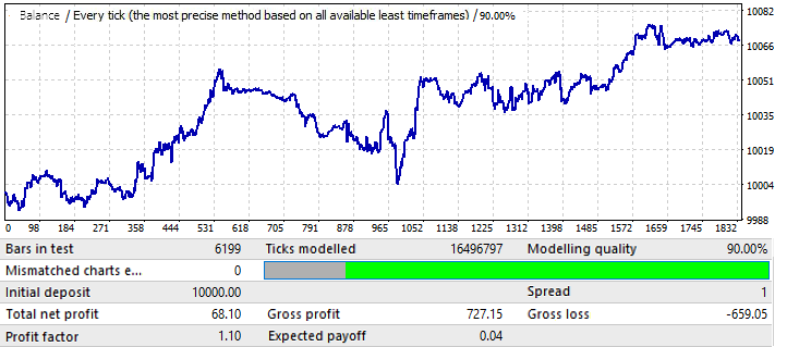
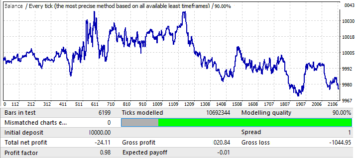
Let us start with EURUSD H1. Testing was performed in the interval 2010.01.01-2020.01.01. Its purpose was to find a global pattern:

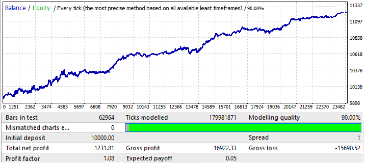
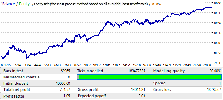
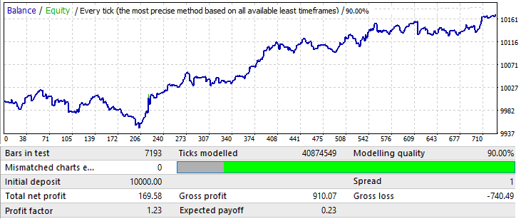
The results are not very attractive, and this is all that we managed to squeeze out of the pair in the given time interval. We can identify a global pattern, although it is not so clear. I used 50 candlesticks in the formula for the brute force. The result is not as good as we could expect, but it is necessary. You will see further what for. Let us test the same segment in the forward period 2020.01.01-2020.11.01, in order to understand its future performance:

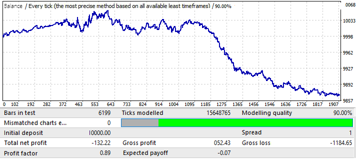
The results is quite understandable. This analysis turned out to be insufficient for trying to profit from the pattern continuation. General, if we analyze global patterns, then the purpose should be to find a pattern that will work for at least several more years, otherwise such an analysis is completely useless. At the beginning of the chart the pattern continues to work, but after six months it is inverted. So such an analysis may be enough for trading for several months, provided we manage to find good enough parameters of the initial test. In this case analysis was performed by the P_Factor value. This parameter is similar to Profit Factor, but it takes values in the range of [0...1] . 1 - 100% of profit. In the first tab, the highest value of this parameter was about 0.029. The average value of all found variants was about 0.02.

The next EURCHF chart:

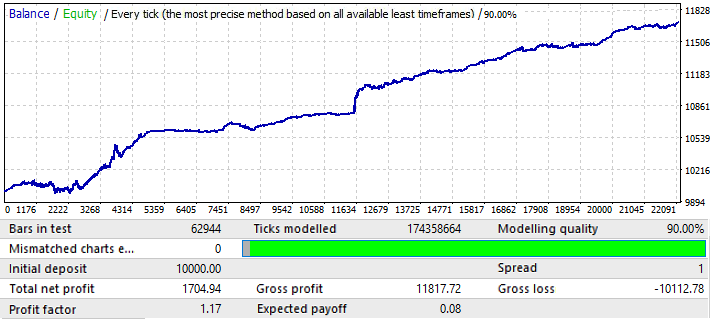
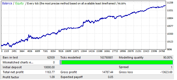
The maximum result for the chart variants on the first tab was around 0.057. Its degree of predictability is 2 times higher than that of the previous chart, which also influenced the final Profit Factor, which is actually 0.09 higher than that of the previous one. Let us see if the improvement in global indicators affected the forward period:

As you can see, the pattern continues throughout the year. It is not very even, and the profit factor is lower. However, we can draw some preliminary conclusions. Actually, the PF is lower because the global test had quite large areas of sharp balance growth, which increased the resulting profit factor. I am sure that if we test it for a few next years, the result will be almost the same. The preliminary conclusion is that an improvement in the chart quality and appearance influenced its performance in the future. So, we got this result by applying the our settings to this particular currency pair. The reason for the waves on the chart can be seen on the global test, where the balance fluctuations have greatly increased in recent years. So, the waves are just a continuation of these fluctuations.

Moving on to the USDJPY chart:

This is the worst chart. Let us check the forward period:

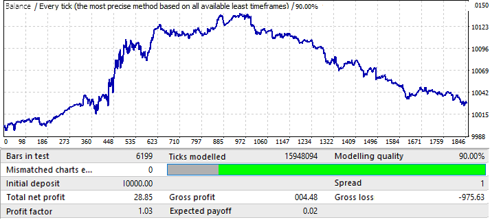
Seems to be in a positive zone, but its second half is very similar to that of the first chart (EURUSD H1), which also started with an upward movement, then reversed and had an almost straight downward movement. So, conclusions are the same here. The final result quality is not high enough. Nevertheless, we could expect a couple of months of profitable trading with this pattern, provided mathematical expectation and profit factor are good enough.

The last chart, USDCHF:

It is not very impressive. Let us have a look at the forward period:

Seems to be similar to other charts, except EURCHF. Its performance is good until the middle of the year, and then it has a reversal and a pattern inversion.

We can draw the following preliminary conclusions:

1. Obviously EURCHF was the best chart
2. EURCHF was better than all other pairs both on the training period and in the forward test
3. In all chart except EURCHF the pattern is preserved until the middle of the year

Based on the above, we can make a conclusion that quality results in the training period directly affect the forward period performance. An increase in the profit factor of the final result can indicate that the result is much less random than that on other charts. This in turn can indicate that we have found a global pattern. As applied to the forex market, we can say that "there is a share of a pattern in any pattern". The stronger the test values, the higher the share.

Now I will try to change the sample size. Let us use 1 year. 2017.01.01-2018.01.01 EURJPY H1. Let us see how the pattern behaves a month ahead in the future:

The chart does not look very good, but the resulting profit factor and the mathematical expectation are higher than those of 10-year variants. The sample is 12 times smaller than the initial variants, however this data should not be ignored.

The forward period is one month: 2018.01.01-2018.02.01:

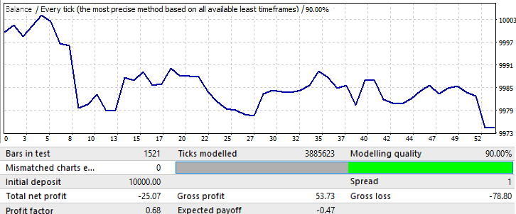
This is only an example to make further reasoning clearer. Here the pattern almost immediately reverses. Unfortunately I could not provide more data. Calculations and software setup take a lot of time. Anyway, this information should be enough for the first analysis.

Data Analysis

After testing the Expert Advisors, we can make some conclusions:

• Expert Advisors that utilize global patterns and that are able to operate in quite a long term, can be created by using a simple number brute force
• The duration of future operation depends directly on the size of the data sample
• The duration of operation depends directly on the test quality in the training area
• When testing for the forward period, the operability of global patterns on all charts remains at least 2-3 months
• The likelihood of finding a pattern that will work for at least a few more years increases when the quality of the final result in the brute force section tends to 100%
• When we search for global patterns, different setting work differently for different currency pairs

As for local patterns, such as a month, the situation is completely different here. In my previous article, I analyzed local patterns, but I did not use the new functions introduced in the program version. Any improvements allow a better understanding of the same questions. As for local patterns:

• Always play the pattern change
• Martingale can be used, by carefully

So, the larger the sample, the longer it will retain its future operability. And vice versa, the smaller the sample, the faster the pattern will invert in the future (of course, provided that there is no forward optimization, which I by the way plan to add later). Pattern inversion in case of a short interval is guaranteed. Based on these conclusions, there are two possible trading types:

1. Exploitation of global patterns
2. Exploitation of local patterns

In the first case, the larger the training area, the longer the pattern will work. However, it is still better to search for new formulas every 2 to 3 months. As for local patterns, searches should be performed every week while the market is frozen. The quality of the results will not be high, but you do not need to worry about the result - at least you will be able to earn some profit.

Now I will try to summarize all the data obtained as a result of my research on different-scale patterns. To do this, I will introducing a function that reflects the expected payoff (math expectation) of a particular order, as well as a function that reflects the profit factor. You can add any other functions that characterize less important metrics. The space of events or a random variable will be all possible variants of event developments in the future. Now we only know the following:

• There are countless possible developments for the "F"-th bar in the future (whether an order is opened on it or not)
• For all options for the future development, in which an order opens on a specific bar, this order will have an expected payoff in points and a profit factor (imagine that you are conducting a test on one bar, only the following bars are always different for each order)
• All these quantities will be different for each formula
• For sections with different future beginning dates (the beginning of the future is the end of the training section) and different training section durations (which is equivalent to different starting dates of the training section), the final sought parameters will take unique values

All these statements can be transformed into mathematical formulas. Here are the formulas:

• MF=MF(T,I,F,S,R) — mathematical expectation of orders on a specific bar in the future.
• PF=PF(T,I,F,S,R)  — profit factor of orders on a specific bar in the future. 
• T  — the duration of the training section (in this case it is the sample size or the number of bars).
• I  — the date of the training section end.
• F  — the bar number in the future, starting with the training end date.
• S  — a unique polynomial or an algorithm (if the pattern is found manually or by another EA).
• R  — the results achieved using a specific polynomial or strategy (the quality of signal optimization); they include the number of trades on the training period and the desired metrics, such as the mathematical expectation, profit factor and other parameters.

Based on the data obtained by brute force on different instruments and different dates, I can draw the above functions on a chart ("F" is used as an argument):

This chart shows 2 unique variants of strategies that were trained in different segments using different settings and achieved different results. There are countless such options, but they all have different duration and quality of the original pattern. This is always followed by a pattern inversion. This rule may not work only for very strong patterns. But even for them there is always a risk that the chart will reverse, maybe in 5 years, but it will reverse. The most stable formulas will be those that are found from the largest sample. If the formulas are found manually and originate from some theory, then such formulas in the future can work indefinitely. However, we have no such guarantees when using brute force or other machine learning methods. All we have is an estimate of operation time, which can only be made based on statistical data. This analysis is possible by using my program, however it cannot be implemented by one person due to the limited time and computing power.

What's Next?

The analysis of global patterns has shown that the power of an ordinary computer is not enough for deep and high-quality analysis of large samples, such as 10 years long or more. Anyway, very large samples should be analyzed in order to ensure high-quality search results. Perhaps if we run the program for a couple of months on a high-performance server, we can find one or two good variants. Therefore, we need to improve efficiency along with an increase in the brute force speed. The possible further development of the program is as follows:

1. Adding the ability to analyze fixed server time windows.
2. Adding the ability to perform analysis on fixed days of the week.
3. Adding the ability to randomly generate time windows.
4. Adding the ability to randomly generate an array of allowed days of the week for trading.
5. Improving the second stage of analysis (optimization tab), in particular, the implementation of multicore computations and correction of optimizer errors.

These changes should greatly increase both the program operation speed and the variability and quality of the found options. They also should provide a convenient toolkit for market analysis.

Conclusions

I hope this article is useful for you. It seems to me that the topic of global patterns in the article is very important. However, it was extremely difficult for me to do this, because the program capabilities are still not enough for this kind of analysis. This would be easier if I had access to 30 cores. To improve the analysis quality, we would need to spend much more time.

Hopefully, it will be possible to access increased computing power in the future. We will continue in the next article. I also provided in this article some mathematics for general understanding, which will be useful when using the program, as well as when searching for patterns manually and optimizing them.

The general ideal of the article was to provide information to those who have not yet managed to achieve even these small results manually. It should help in understanding the basics of underlying ideas used when developing robots.

It seems to me not so important how you find a patter, manually or using some software. If a pattern has some profitable results, we can consider it a working pattern. Some pattern parameters give us some predictions. This may be a near-future prediction, but it still can be enough to earn. However, if you have found a pattern, it does not mean that the same pattern will work in the future. To check it, you will need a very large sample with very good trading results throughout the sample and with a sufficient number of orders considering the sample size. Apart from finding a pattern, there is another problem - estimating it possible future operation time. This question is fundamental, in my opinion. What is the point in finding a pattern if we do not understand how long and how well it will work. Anyone can use my program. It is available in the article attachment. Please PM me for specific setup questions.