Neural Networks in Trading: Mask-Attention-Free Approach to Price Movement Forecasting

MetaTrader 5 — Trading systems | 12 May 2025, 15:00

1 084

Dmitriy Gizlyk

Introduction

We continue our exploration using the point cloud processing method. In the previous article, we introduced the SPFormer method. Its authors developed a comprehensive algorithm based on the Transformer architecture. Several layers of the Transformer decoder utilize a fixed number of object queries, enabling iterative processing of global features and direct object prediction. SPFormer does not require post-processing to eliminate duplicates, as a one-to-one bipartite matching strategy is employed during training. Moreover, the object masks generated in the final layer are used to guide cross-attention.

However, the authors of the paper "Mask-Attention-Free Transformer for 3D Instance Segmentation" note that current Transformer-based methods suffer from slow convergence. Through analysis of the baseline method, they identified that this issue may stem from the low quality of the initial masks. Specifically, the initial object masks are generated by mapping the similarity between initial object queries and per-point mask features. Poor-quality initial masks increase the complexity of training, thereby slowing down convergence.

To address the low completeness of initial masks, the authors propose a novel algorithm, Mask-Attention-Free Transformer (MATF), which abandons the mask attention design and instead introduces an auxiliary center regression task to guide cross-attention. To enable center regression, the authors developed a series of components that take point positions into account. First, they add a set of learnable positional queries, each representing the position of a corresponding content query. These query positions are densely distributed throughout the learning space. A constraint is also introduced to ensure that each query focuses on its local region. As a result, queries can effectively capture objects in the scene with higher distinctiveness, which is critical for reducing training complexity and accelerating convergence.

In addition, the authors of MATF propose contextual relative position encoding for cross-attention. Compared to the attention mask used in previous works, this solution is more flexible, as attention weights are adjusted based on relative positions rather than a rigid mask. The query positions are updated iteratively to achieve more accurate representations.

The experimental results presented in the paper demonstrate that MATF delivers superior performance across various datasets.

1. The MATF algorithm

The SPFormer algorithm represents a fully end-to-end pipeline that allows object queries to directly generate instance predictions. Using Transformer decoders, a fixed number of object queries aggregate global object information from the analyzed point cloud. Moreover, SPFormer leverages object masks to guide cross-attention, requiring queries to attend only to masked features. However, in the early stages of training, these masks are of low quality. This hampers performance in subsequent layers and increases the overall training complexity.

To address this, the authors of the MAFT method introduce an auxiliary center regression task to guide instance segmentation. Initially, global positions 𝒫 are selected from the raw point cloud, and global object features ℱ are extracted via a backbone network. These can be voxels or superpoints. In addition to the content queries 𝒬0c, the authors of MAFT introduces a fixed number of positional queries 𝒬0p, representing normalized object centers. While 𝒬0p is initialized randomly, 𝒬0c starts with zero values. The core objective is to allow the positional queries to guide the corresponding contextual queries in cross-attention, followed by iterative refinement of both query sets to predict object centers, classes, and masks.

To effectively solve the object center regression task and improve the generation of initial object masks, the authors of MAFT propose a series of architectural components that account for point positions.

Unlike prior approaches, an additional set of positional queries 𝒬0p is introduced. Given that point ranges vary significantly across scenes, the initial position queries are stored in normalized form as learnable parameters, followed by a sigmoid activation function.

Notably, these initial position queries are densely distributed throughout the target space. Furthermore, each query aggregates objects from its corresponding local region. This design facilitates the ability of the initial queries to capture scene objects with high recall. It addresses the problem of low memorability caused by poor-quality initial instance masks and reduces the training complexity in subsequent layers.

In addition to absolute position encoding, MAFT employs contextual relative position encoding in the cross-attention mechanism. To achieve this, relative positions 𝐫 between positional queries 𝒬tp and global positions 𝒫 are first computed and then quantized into discrete integers 𝐫'. These discrete relative positions are used as indices to retrieve corresponding values from a positional encoding table.

Next, the relative position encoding 𝐟pos is multiplied with Query 𝐟q or Key features 𝐟k in the cross-attention module. The result is then added to the cross-attention weights, followed by a Softmax function.

It is worth noting that relative positional encoding provides greater flexibility and robustness to errors compared to masked attention. In essence, it functions as a soft mask that flexibly adjusts attention weights rather than applying rigid masking. Another advantage is that it integrates semantic information and can selectively capture local context. This is achieved through the interaction between relative positions and semantic features.

As contextual queries in the decoder layers are continuously updated, maintaining fixed positional queries throughout decoding is suboptimal. Since the initial positional queries are static, it is beneficial to adapt them to the specific input scene in subsequent layers. To achieve this, the authors iteratively refine the positional queries based on the content queries. Specifically, an MLP is used to predict the center offset Δpt from the updated contextual query 𝒬t+1c. This offset is then added to the previous positional query 𝒬tp.

The original visualization of the MAFT method from the above paper is shown below.

2. Implementation in MQL5

Having explored the theoretical foundations of the Mask-Attention-Free Transformer method, we now move on to the practical part of our article, where we implement our interpretation of the proposed approaches using MQL5. We begin by extending the OpenCL program.

2.1 Extending the OpenCL Program

We start by constructing the relative positional encoding algorithm. On one hand, the algorithm is relatively simple. We only need to calculate the distance between two points. Moreover, the authors compute the distance along each coordinate axis individually. On the other hand, the MAFT authors perform quantization of the resulting offsets, which are then used to index into a learnable parameter table. We opted to slightly optimize the original solution. Our implementation is based on the assumption that the greatest influence comes from points located in close proximity to the query being analyzed. Following this logic, we first calculate the distance S between two points in an N-dimensional space. And then compute the positional bias coefficient kpb using the following formula:

It is clear that the distance between any two points is always greater than or equal to 0. If the points coincide, the coefficient equals 1. As the distance increases, the relative positional encoding coefficient approaches 0.

The implementation of the proposed algorithm is provided in the CalcPositionBias kernel. The kernel parameters include pointers to three global data buffers: 2 of them contain the input data. The third is intended for storing the results. Additionally, we specify the dimensionality of the feature vector for a single element.

Note that to correctly compute the distance between two vectors, they must be projected onto the same subspace. This implies that the feature vectors in both input tensors must have the same dimensionality.

__kernel void CalcPositionBias(__global const float *data1,
                               __global const float *data2,
                               __global float *result,
                               const int dimension
                              )
  {
   const size_t idx1 = get_global_id(0);
   const size_t idx2 = get_global_id(1);
   const size_t total1 = get_global_size(0);
   const size_t total2 = get_global_size(1);

We plan to launch the kernel in a two-dimensional space of tasks, each of which is equal to the number of elements in the corresponding tensor of the original data. In the kernel body, we immediately identify the current thread in both dimensions of the task space.

In the next step, we determine the offset into the data buffers.

   const int shift1 = idx1 * dimension;
   const int shift2 = idx2 * dimension;
   const int shift_out = idx1 * total2 + idx2;

After completing the preparatory stage, we proceed to the execution of calculations. Here, we first organize a loop for calculating the distance between the analyzed vectors.

   float res = 0;
   for(int i = 0; i < dimension; i++)
      res = pow(data1[shift1 + i] - data2[shift2 + i], 2.0f);
   res = sqrt(res);

And then we compute the relative bias coefficient.

   res = 1.0f / exp(res);
   if(isnan(res) || isinf(res))
      res = 0;
//---
   result[shift_out] = res;
  }

We then write the calculated value to the corresponding element in the results buffer.

Note that none of the obtained coefficients are negative. This means that we are not masking out any elements in the input sequence. On the contrary, our implementation emphasizes elements that are spatially closest to the query.

At this stage, we have computed the relative positional bias coefficients. The next step is to integrate them into our cross-attention mechanism. However, before we proceed with the implementation, I would like to draw your attention to an important detail. Take a closer look at the authors' visualization of the MAFT method shown above. Particularly pay attention the flow of scene representation information. What stands out is the authors' approach to positional encoding within the scene representation. Specifically, positional encoding is applied only to the Key entities. The Value entities remain unaffected by positional encoding. This appears to be a deliberate choice to ensure that attention weights are computed taking into account positional encoding. But at the same time, they do not distort the actual feature descriptors of the scene elements. Consequently, the Key and Value tensors must be generated from different sources. In practical terms, we must first generate the Value tensor from the raw input representation. Then we add positional encoding to the original data. Only then can we obtain the Key tensor.

Why am I highlighting this now? The reasoning above implies that we must separate the Key and Value entities into distinct tensors. We can design a new attention kernel that accounts for this architectural nuance. This approach will also allow us to avoid concatenating two tensors, which we previously had to perform.

To implement the attention algorithm, we will create a kernel called MHPosBiasAttentionOut. This kernel accepts a substantial list of global data buffers, many of which are familiar from our previous attention mechanism implementations. Additionally, we pass a pointer to the buffer of relative positional bias indices pos_bias. We have also designed this kernel to optionally support standard attention computation without positional bias. This functionality can be enabled and disabled using the use_pos_bias parameter.

__kernel void MHPosBiasAttentionOut(__global const float *q,         ///<[in] Matrix of Querys
                                    __global const float *k,         ///<[in] Matrix of Keys
                                    __global const float *v,         ///<[in] Matrix of Values
                                    __global float *score,           ///<[out] Matrix of Scores
                                    __global const float *pos_bias,  ///<[in] Position Bias
                                    __global float *out,             ///<[out] Matrix of attention
                                    const int dimension,             ///< Dimension of Key
                                    const int heads_kv,
                                    const int use_pos_bias
                                   )
  {
//---
   const int q_id = get_global_id(0);
   const int k_id = get_global_id(1);
   const int h = get_global_id(2);
   const int qunits = get_global_size(0);
   const int kunits = get_global_size(1);
   const int heads = get_global_size(2);

As before, we plan to run this kernel in a three-dimensional task space. The first two indicate the number of elements in the sequences being analyzed, and the third dimension of the task space indicates the number of attention heads used. The kernel algorithm starts by identifying the current thread in all three dimensions of the task space.

Next, we define all the necessary constants.

   const int h_kv = h % heads_kv;
   const int shift_q = dimension * (q_id * heads + h);
   const int shift_kv = dimension * (heads_kv * k_id + h_kv);
   const int shift_s = kunits * (q_id *  heads + h) + k_id;
   const int shift_pb = q_id * kunits + k_id;
   const uint ls = min((uint)get_local_size(1), (uint)LOCAL_ARRAY_SIZE);
   float koef = sqrt((float)dimension);
   if(koef < 1)
      koef = 1;

And then we create an array of data in local memory for exchanging data between threads of the local group.

   __local float temp[LOCAL_ARRAY_SIZE];

This completes the preparatory work stage, and we move directly to the calculations. The calculation process largely repeats the classical algorithm. We only add relative positional bias where necessary. The necessity of their use is controlled by the value of the use_pos_bias parameter.

First, we calculate the sum of the exponential values of the attention coefficients. At the first stage, each thread of the local group calculates its part. Then it saves the result in the corresponding element of the local data array.

//--- sum of exp
   uint count = 0;
   if(k_id < ls)
     {
      temp[k_id] = 0;
      do
        {
         if(q_id >= (count * ls + k_id))
            if((count * ls) < (kunits - k_id))
              {
               float sum = 0;
               int sh_k = dimension * heads_kv * count * ls;
               for(int d = 0; d < dimension; d++)
                  sum = q[shift_q + d] * k[shift_kv + d + sh_k];
               sum = exp(sum / koef);
               if(isnan(sum))
                  sum = 0;
               temp[k_id] = temp[k_id] + sum + (use_pos_bias > 0 ? pos_bias[shift_pb + count * ls] : 0);
              }
         count++;
        }
      while((count * ls + k_id) < kunits);
     }
   barrier(CLK_LOCAL_MEM_FENCE);

Please note that the sum we calculate must include the sum of the positional bias coefficients.

Next, we sum the value of the elements of the local array.

   count = min(ls, (uint)kunits);
//---
   do
     {
      count = (count + 1) / 2;
      if(k_id < ls)
         temp[k_id] += (k_id < count && (k_id + count) < kunits ? temp[k_id + count] : 0);
      if(k_id + count < ls)
         temp[k_id + count] = 0;
      barrier(CLK_LOCAL_MEM_FENCE);
     }
   while(count > 1);

After calculating the total sum, we determine and store the normalized values of the dependence coefficients taking into account the positional bias coefficients.

//--- score
   float sum = temp[0];
   float sc = 0;
   if(q_id >= (count * ls + k_id))
      if(sum != 0)
        {
         for(int d = 0; d < dimension; d++)
            sc = q[shift_q + d] * k[shift_kv + d];
         sc = (exp(sc / koef) + (use_pos_bias > 0 ? pos_bias[shift_pb] : 0)) / sum;
         if(isnan(sc))
            sc = 0;
        }
   score[shift_s] = sc;
   barrier(CLK_LOCAL_MEM_FENCE);

The obtained attention coefficients allow us to calculate the final values of multi-headed attention for each element of the analyzed sequence.

//--- out
   for(int d = 0; d < dimension; d++)
     {
      uint count = 0;
      if(k_id < ls)
         do
           {
            if((count * ls) < (kunits - k_id))
              {
               int sh_v = 2 * dimension * heads_kv * count * ls;
               float sum =
                  v[shift_kv + d + sh_v] * (count == 0 ? sc : score[shift_s + count * ls]);
               if(isnan(sum))
                  sum = 0;
               temp[k_id] = (count > 0 ? temp[k_id] : 0) + sum;
              }
            count++;
           }
         while((count * ls + k_id) < kunits);
      barrier(CLK_LOCAL_MEM_FENCE);
      //---
      count = min(ls, (uint)kunits);
      do
        {
         count = (count + 1) / 2;
         if(k_id < ls)
            temp[k_id] += (k_id < count && (k_id + count) < kunits ? temp[k_id + count] : 0);
         if(k_id + count < ls)
            temp[k_id + count] = 0;
         barrier(CLK_LOCAL_MEM_FENCE);
        }
      while(count > 1);
      //---
      out[shift_q + d] = temp[0];
     }
  }

Next, we proceed to implement the backpropagation algorithm in the MHPosBiasAttentionInsideGradients kernel. It is worth recalling that when distributing error gradients through a summation operation, the gradient is typically propagated in full to both summands. The use of a learning rate significantly less than 1 more than compensates for the potential overcounting of the error. Another key point to consider is that the calculation of relative positional bias coefficients is based solely on the actual spatial arrangement of points. These actually represent the raw input data. So, these computations are not influenced by model parameters. The calculation process itself includes no learnable parameters. Consequently, propagating gradients to the tensor of relative positional bias coefficients is illogical. Therefore, we exclude this step from the backpropagation process.

Taking these considerations into account, we arrive at a classical gradient distribution approach for the attention block. However, we developed a new kernel because, as discussed earlier, we separated the Key and Value entities into distinct data buffers. You can review the implementation of the MHPosBiasAttentionInsideGradients backpropagation kernel in the attached file. With this, we conclude our work on the OpenCL component.

2.2 Creating the MAFT Class

The next phase of our work involves creating a new object that encapsulates our interpretation of the techniques proposed by the authors of the Mask-Attention-Free Transformer method. For this purpose, we introduce a new class named CNeuronMAFT.

The MAFT algorithm is built upon the previously discussed SPFormer architecture. Similarly, our implementation will leverage the groundwork laid in the CNeuronSPFormer class. However, the scale and scope of changes render inheritance from that class impractical. As a result, our new object will inherit directly from the base fully connected layer class CNeuronBaseOCL. The structure of the new class is shown below.

class CNeuronMAFT   : public CNeuronBaseOCL
  {
protected:
   uint              iWindow;
   uint              iUnits;
   uint              iHeads;
   uint              iSPWindow;
   uint              iSPUnits;
   uint              iSPHeads;
   uint              iWindowKey;
   uint              iLayers;
   uint              iLayersSP;
   //---
   CLayer            cSuperPoints;
   CLayer            cQuery;
   CLayer            cQPosition;
   CLayer            cQKey;
   CLayer            cQValue;
   CLayer            cMHSelfAttentionOut;
   CLayer            cSelfAttentionOut;
   CLayer            cSPKey;
   CLayer            cSPValue;
   CArrayInt         cScores;
   CArrayInt         cPositionBias;
   CLayer            cMHCrossAttentionOut;
   CLayer            cCrossAttentionOut;
   CLayer            cResidual;
   CLayer            cFeedForward;
   CBufferFloat      cTempSP;
   CBufferFloat      cTempQ;
   CBufferFloat      cTempCrossK;
   CBufferFloat      cTempCrossV;
   //---
   virtual bool      CreateBuffers(void);
   virtual bool      CalcPositionBias(CBufferFloat *pos_q, CBufferFloat *pos_k, const int pos_bias,
                                      const int units,
                                      const int units_kv,
                                      const int dimension);
   virtual bool      AttentionOut(CNeuronBaseOCL *q, CNeuronBaseOCL *k, CNeuronBaseOCL *v,
                                  const int scores, CNeuronBaseOCL *out, const int pos_bias,
                                  const int units,
                                  const int heads,
                                  const int units_kv,
                                  const int heads_kv,
                                  const int dimension,
                                  const bool use_pos_bias);
   virtual bool      AttentionInsideGradients(CNeuronBaseOCL *q, CNeuronBaseOCL *k, CNeuronBaseOCL *v,
         const int scores, CNeuronBaseOCL *out,
         const int units, const int heads,
         const int units_kv, const int heads_kv,
         const int dimension);
   //---
   virtual bool      feedForward(CNeuronBaseOCL *NeuronOCL) override;
   //---
   virtual bool      calcInputGradients(CNeuronBaseOCL *NeuronOCL) override;
   virtual bool      updateInputWeights(CNeuronBaseOCL *NeuronOCL) override;

public:
                     CNeuronMAFT(void) {};
                    ~CNeuronMAFT(void) {};
   //---
   virtual bool      Init(uint numOutputs, uint myIndex, COpenCLMy *open_cl,
                          uint window, uint window_key, uint units_count, uint heads,
                          uint window_sp, uint units_sp, uint heads_sp,
                          uint layers, uint layers_to_sp,
                          ENUM_OPTIMIZATION optimization_type, uint batch);
   //---
   virtual int       Type(void) override   const   {  return defNeuronMAFT; }
   //---
   virtual bool      Save(int const file_handle) override;
   virtual bool      Load(int const file_handle) override;
   //---
   virtual bool      WeightsUpdate(CNeuronBaseOCL *source, float tau) override;
   virtual void      SetOpenCL(COpenCLMy *obj) override;
  };

In the presented structure, we observe the familiar set of overridable virtual methods along with a large number of internal objects. Some of these internal components repeat those used previously, while others are entirely new. We will become familiar with the functionality of each as we proceed with the implementation of the CNeuronMAFT class methods.

As before, all internal objects are declared statically, allowing us to leave the class constructor and destructor empty. Initialization of both inherited and newly declared components is handled in the Init method.

bool CNeuronMAFT::Init(uint numOutputs, uint myIndex, COpenCLMy *open_cl,
                       uint window, uint window_key, uint units_count,
                       uint heads, uint window_sp, uint units_sp, uint heads_sp,
                       uint layers, uint layers_to_sp,
                       ENUM_OPTIMIZATION optimization_type, uint batch)
  {
   if(!CNeuronBaseOCL::Init(numOutputs, myIndex, open_cl, window * units_count, optimization_type, batch))
      return false;

The parameters of this method include key constants defining the architecture of the object being created. It can be noticed here that the parameters of this method are completely borrowed from the relevant method of the CNeuronSPFormer class. This is consistent with the inheritance-based design philosophy we are following. However, the actual logic of the method has not undergone major changes.

In the body of the method, we first call the same method of the parent class, which implements primary control over the received parameters and initializes the inherited objects. After that, we save the resulting constants in the internal variables of the class.

   iWindow = window;
   iUnits = units_count;
   iHeads = heads;
   iSPUnits = units_sp;
   iSPWindow = window_sp;
   iSPHeads = heads_sp;
   iWindowKey = window_key;
   iLayers = MathMax(layers, 1);
   iLayersSP = MathMax(layers_to_sp, 1);

The next step is to initialize the objects for generating learnable queries of objects and their positional encoding. The authors of the MAFT method proposed to initialize queries with zero values. We can do the same. To do this, we reset the query generation parameters.

   CNeuronBaseOCL *base = new CNeuronBaseOCL();
   if(!base)
      return false;
   if(!base.Init(iWindow * iUnits, 0, OpenCL, 1, optimization, iBatch))
      return false;
   CBufferFloat *buf = base.getOutput();
   if(!buf || !buf.BufferInit(1, 1) || !buf.BufferWrite())
      return false;
   buf = base.getWeights();
   if(!buf || !buf.BufferInit(buf.Total(), 0) ||
      !buf.BufferWrite())
      return false;
   if(!cQuery.Add(base))
      return false;
   base = new CNeuronBaseOCL();
   if(!base || !base.Init(0, 1, OpenCL, iWindow * iUnits, optimization, iBatch))
      return false;
   if(!cQuery.Add(base))
      return false;

We also add a learnable positional encoding initialized with random values.

   CNeuronLearnabledPE *pe = new CNeuronLearnabledPE();
   if(!pe || !pe.Init(0, 2, OpenCL, base.Neurons(), optimization, iBatch))
      return false;
   if(!cQuery.Add(pe))
      return false;

It should be said that positional coding goes as a separate flow of information through the entire MAFT algorithm. Therefore, we will provide it as separate objects.

   if(!base || !base.Init(0, 3, OpenCL, pe.Neurons(), optimization, iBatch))
      return false;
   if(!base.SetOutput(pe.getOutput()))
      return false;
   if(!cQPosition.Add(base))
      return false;

The next stage is primary data processing. And here we borrow the Superpoint approach, which was presented in the SPFormer method.

//--- Init SuperPoints
   int layer_id = 4;
   for(int r = 0; r < 4; r++)
     {
      if(iSPUnits % 2 == 0)
        {
         iSPUnits /= 2;
         CResidualConv *residual = new CResidualConv();
         if(!residual)
            return false;
         if(!residual.Init(0, layer_id, OpenCL, 2 * iSPWindow, iSPWindow, iSPUnits, optimization, iBatch))
            return false;
         if(!cSuperPoints.Add(residual))
            return false;
        }
      else
        {
         iSPUnits--;
         CNeuronConvOCL *conv = new CNeuronConvOCL();
         if(!conv.Init(0, layer_id, OpenCL, 2 * iSPWindow, iSPWindow, iSPWindow, iSPUnits, 1,
                                                                        optimization, iBatch))
            return false;
         if(!cSuperPoints.Add(conv))
            return false;
        }
      layer_id++;
     }

Please note here that the presented implementation allows the use of tensors of different dimensions for cross-attention. However, this is unacceptable for the proposed algorithm of relative positional offset coefficients. Therefore, we add a superpoint projection layer to the learnable query space.

   CNeuronConvOCL *conv = new CNeuronConvOCL();
   if(!conv.Init(0, layer_id, OpenCL, iSPWindow, iSPWindow, iWindow, iSPUnits, 1, optimization, iBatch))
      return false;
   if(!cSuperPoints.Add(conv))
      return false;
   layer_id++;

And we add a layer of positional encoding.

   pe = new CNeuronLearnabledPE();
   if(!pe || !pe.Init(0, layer_id, OpenCL, conv.Neurons(), optimization, iBatch))
      return false;
   if(!cSuperPoints.Add(pe))
      return false;
   layer_id++;

Please note that at this point, we have deviated a little from the original algorithm proposed by the authors of the MAFT method. In their work, they used voxelization of a point cloud based on the original coordinates. Instead of this, we used fully learnable positional encoding, thereby allowing the model to learn the optimal positions of each element of the input sequence.

After completing the work on the primary processing of the source data, we organize a loop through the internal layers of the Decoder.

//--- Inside layers
   for(uint l = 0; l < iLayers; l++)
     {
      //--- Self-Attention
      //--- Query
      conv = new CNeuronConvOCL();
      if(!conv || !conv.Init(0, layer_id, OpenCL, iWindow, iWindow, iWindowKey * iHeads, iUnits, 1, 
                                                                              optimization, iBatch))
         return false;
      if(!cQuery.Add(conv))
         return false;
      layer_id++;

Note here that the authors of MAFT use a classic layout: Self-Attention -> Cross-Attention -> Feed Forward. However, the authors of the SPFormer method swapped Self-Attention and Cross-Attention.

First, we generate Query entities. Then we add Key and Value.

      //--- Key
      conv = new CNeuronConvOCL();
      if(!conv || !conv.Init(0, layer_id, OpenCL, iWindow, iWindow, iWindowKey * iHeads, iUnits, 1, 
                                                                              optimization, iBatch))
         return false;
      if(!cQKey.Add(conv))
         return false;
      layer_id++;
      //--- Value
      conv = new CNeuronConvOCL();
      if(!conv || !conv.Init(0, layer_id, OpenCL, iWindow, iWindow, iWindowKey * iHeads, iUnits, 1, 
                                                                               optimization, iBatch))
         return false;
      if(!cQValue.Add(conv))
         return false;
      layer_id++;

In this case, we expect to use a small number of learnable queries. Therefore, we do not reduce the number of heads for Key-Value and generate new entities on each internal layer.

We pass the generated entities to the multi-headed attention block without using positional bias coefficients.

      //--- Multy-Heads Attention Out
      base = new CNeuronBaseOCL();
      if(!base || !base.Init(0, layer_id, OpenCL, iWindowKey * iHeads * iUnits, optimization, iBatch))
         return false;
      if(!cMHSelfAttentionOut.Add(base))
         return false;
      layer_id++;

We add a layer of scaling the results of multi-headed attention.

      //--- Self-Attention Out
      conv = new CNeuronConvOCL();
      if(!conv || !conv.Init(0, layer_id, OpenCL, iWindowKey * iHeads, iWindowKey * iHeads, iWindow,
                                                                     iUnits, 1, optimization, iBatch))
         return false;
      if(!cSelfAttentionOut.Add(conv))
         return false;
      layer_id++;

At the end of the Self-Attention block, following the classical Transformer algorithm, we add a layer of residual connections.

      //--- Residual
      base = new CNeuronBaseOCL();
      if(!base || !base.Init(0, layer_id, OpenCL, iWindow * iUnits, optimization, iBatch))
         return false;
      if(!cResidual.Add(base))
         return false;
      layer_id++;

Next, we build the objects of the cross-attention block. We start with the Query entity tensor.

      //--- Cross-Attention
      //--- Query
      conv = new CNeuronConvOCL();
      if(!conv || !conv.Init(0, layer_id, OpenCL, iWindow, iWindow, iWindowKey * iHeads, iUnits, 1,
                                                                              optimization, iBatch))
         return false;
      if(!cQuery.Add(conv))
         return false;
      layer_id++;

Then we add tensors for the Key and Value entities. This time we follow the user's instructions to reduce attention heads and alternate layers.

      if(l % iLayersSP == 0)
        {
         //--- Key
         conv = new CNeuronConvOCL();
         if(!conv || !conv.Init(0, layer_id, OpenCL, iWindow, iWindow, iWindowKey * iSPHeads, iSPUnits, 1,
                                                                                     optimization, iBatch))
            return false;
         if(!cSPKey.Add(conv))
            return false;
         layer_id++;
         //--- Value
         conv = new CNeuronConvOCL();
         if(!conv || !conv.Init(0, layer_id, OpenCL, iWindow, iWindow, iWindowKey * iSPHeads, iSPUnits, 1, 
                                                                                     optimization, iBatch))
            return false;
         if(!cSPValue.Add(conv))
            return false;
         layer_id++;
        }

We add a layer of results from multi-headed attention.

      //--- Multy-Heads Attention Out
      base = new CNeuronBaseOCL();
      if(!base || !base.Init(0, layer_id, OpenCL, iWindowKey * iHeads * iUnits, optimization, iBatch))
         return false;
      if(!cMHCrossAttentionOut.Add(base))
         return false;
      layer_id++;

It is then scaled by adding residual connections.

      //--- Cross-Attention Out
      conv = new CNeuronConvOCL();
      if(!conv || !conv.Init(0, layer_id, OpenCL, iWindowKey * iHeads, iWindowKey * iHeads, iWindow,
                                                                    iUnits, 1, optimization, iBatch))
         return false;
      if(!cCrossAttentionOut.Add(conv))
         return false;
      layer_id++;
      //--- Residual
      base = new CNeuronBaseOCL();
      if(!base || !base.Init(0, layer_id, OpenCL, iWindow * iUnits, optimization, iBatch))
         return false;
      if(!cResidual.Add(base))
         return false;
      layer_id++;

The decoder is completed by the FeedForward block, to which we also add residual connections.

      //--- Feed Forward
      conv = new CNeuronConvOCL();
      if(!conv || !conv.Init(0, layer_id, OpenCL, iWindow, iWindow, 4 * iWindow, iUnits, 1, 
                                                                         optimization, iBatch))
         return false;
      conv.SetActivationFunction(LReLU);
      if(!cFeedForward.Add(conv))
         return false;
      layer_id++;
      conv = new CNeuronConvOCL();
      if(!conv || !conv.Init(0, layer_id, OpenCL, 4 * iWindow, 4 * iWindow, iWindow, iUnits, 1, 
                                                                         optimization, iBatch))
         return false;
      if(!cFeedForward.Add(conv))
         return false;
      layer_id++;
      //--- Residual
      base = new CNeuronBaseOCL();
      if(!base || !base.Init(0, layer_id, OpenCL, iWindow * iUnits, optimization, iBatch))
         return false;
      if(!base.SetGradient(conv.getGradient()))
         return false;
      if(!cResidual.Add(base))
         return false;
      layer_id++;

Now, we just need to add MLP corrections for positional encoding of learnable queries.

      //--- Delta position
      conv = new CNeuronConvOCL();
      if(!conv || !conv.Init(0, layer_id, OpenCL, iWindow, iWindow, iWindow, iUnits, 1, optimization, iBatch))
         return false;
      conv.SetActivationFunction(SIGMOID);
      if(!cQPosition.Add(conv))
         return false;
      layer_id++;
      base = new CNeuronBaseOCL();
      if(!base || !base.Init(0, layer_id, OpenCL, conv.Neurons(), optimization, iBatch))
         return false;
      if(!base.SetGradient(conv.getGradient()))
         return false;
      if(!cQPosition.Add(base))
         return false;
      layer_id++;
     }

Then we move on to the next iteration of the loop, creating objects of the new internal layer of the Decoder.

After successful initialization of objects of all internal layers of the Decoder, we replace pointers to error gradient buffers and return the boolean result indicating success to the calling program.

   base = cResidual[iLayers * 3 - 1];
   if(!SetGradient(base.getGradient()))
      return false;
//---
   SetOpenCL(OpenCL);
//---
   return true;
  }

It should be added that the initialization of auxiliary data buffers is moved to a separate method CreateBuffers, which I suggest you study yourself.

The full implementation of this class and all its methods can be found in the attachment.

After initializing the internal objects, we move on to constructing a feed-forward pass algorithm in the feedForward method. In the parameters of this method, we receive a pointer to the source data object.

bool CNeuronMAFT::feedForward(CNeuronBaseOCL *NeuronOCL)
  {
//--- Superpoints
   CNeuronBaseOCL *superpoints = NeuronOCL;
   int total_sp = cSuperPoints.Total();
   for(int i = 0; i < total_sp; i++)
     {
      if(!cSuperPoints[i] ||
         !((CNeuronBaseOCL*)cSuperPoints[i]).FeedForward(superpoints))
         return false;
      superpoints = cSuperPoints[i];
     }

We immediately use the resulting object while generating superpoint features. For this we will use a nested model cSuperPoints.

The last layer of this model is the positional encoding layer.

Next, we generate learnable queries with positional encoding.

//--- Query
   CNeuronBaseOCL *inputs = NULL;
   for(int i = 0; i < 2; i++)
     {
      inputs = cQuery[i + 1];
      if(!inputs ||
         !inputs.FeedForward(cQuery[i]))
         return false;
     }

Then, we create local variables to temporarily store pointers to objects.

   CNeuronBaseOCL *query = NULL, *key = NULL, *value = NULL, *base = NULL;

We organize a loop through the internal layers of the Decoder.

//--- Inside layers
   for(uint l = 0; l < iLayers; l++)
     {
      //--- Self-Atention
      query = cQuery[l * 2 + 3];
      if(!query || !query.FeedForward(inputs))
         return false;
      key = cQKey[l];
      if(!key || !key.FeedForward(inputs))
         return false;
      value = cQValue[l];
      if(!value || !value.FeedForward(inputs))
         return false;

Here we first organize operations of the Self-Attention block for the learnable queries with positional encoding. To do this, we first generate the necessary entities, which we pass to the multi-headed attention block.

      if(!AttentionOut(query, key, value, cScores[l * 2], cMHSelfAttentionOut[l], -1, 
                                   iUnits, iHeads, iUnits, iHeads, iWindowKey, false))
         return false;

Then we scale the obtained results and add residual connections.

      base = cSelfAttentionOut[l];
      if(!base || !base.FeedForward(cMHSelfAttentionOut[l]))
         return false;
      value = cResidual[l * 3];
      if(!value ||
         !SumAndNormilize(inputs.getOutput(), base.getOutput(), value.getOutput(), iWindow, true, 0, 0, 0, 1))
         return false;
      inputs = value;

As a separate thread, we add positional coding.

      value = cQPosition[l * 2];
      if(!value ||
         !SumAndNormilize(inputs.getOutput(), value.getOutput(),inputs.getOutput(), iWindow, false, 0, 0, 0, 1))
         return false;

After that we move on to the cross-attention block. But first, let's define the coefficients of relative positional bias.

      //--- Calc Position bias
      if(!CalcPositionBias(value.getOutput(),
                           ((CNeuronLearnabledPE*)superpoints).GetPE(), cPositionBias[l],
                           iUnits, iSPUnits, iWindow))
         return false;

Next, we generate a Query entity from the positional query tensor taking into account positional encoding.

      //--- Cross-Attention
      query = cQuery[l * 2 + 4];
      if(!query || !query.FeedForward(inputs))
         return false;

As for the operations of the Key and Value entities are full of nuances. First, new tensors are generated only when necessary.

      key = cSPKey[l / iLayersSP];
      value = cSPValue[l / iLayersSP];
      if(l % iLayersSP == 0)
        {
         if(!key || !key.FeedForward(superpoints))
            return false;
         if(!value || !value.FeedForward(cSuperPoints[total_sp - 2]))
            return false;
        }

Second, the Key entity is generated from the data of the last cSuperPoints layer, which contains positional encoding. To generate Value, we use the penultimate layer which does not have positional encoding.

We pass the resulting entities to the multi-headed attention block without using positional bias coefficients.

      if(!AttentionOut(query, key, value, cScores[l * 2 + 1], cMHCrossAttentionOut[l], cPositionBias[l], 
                                                  iUnits, iHeads, iSPUnits, iSPHeads, iWindowKey, true))
         return false;

After that we scale the obtained data and add residual connections.

      base = cCrossAttentionOut[l];
      if(!base || !base.FeedForward(cMHCrossAttentionOut[l]))
         return false;
      value = cResidual[l * 3 + 1];
      if(!value ||
         !SumAndNormilize(inputs.getOutput(), base.getOutput(), value.getOutput(), iWindow, true, 0, 0, 0, 1))
         return false;
      inputs = value;

At the end of the Decoder, we pass the data through a FeedForward block followed by residual connections.

      //--- Feed Forward
      base = cFeedForward[l * 2];
      if(!base || !base.FeedForward(inputs))
         return false;
      base = cFeedForward[l * 2 + 1];
      if(!base || !base.FeedForward(cFeedForward[l * 2]))
         return false;
      value = cResidual[l * 3 + 2];
      if(!value ||
         !SumAndNormilize(inputs.getOutput(), base.getOutput(), value.getOutput(), iWindow, true, 0, 0, 0, 1))
         return false;
      inputs = value;

At this stage, we have completed the operations of one Decoder layer, but we still have to adjust the positional encoding data of the learnable queries. To do this, we will generate a position deviation based on the data received and add it to the existing values.

      //--- Delta Query position
      base = cQPosition[l * 2 + 1];
      if(!base ||
         !base.FeedForward(inputs))
         return false;
      value = cQPosition[(l + 1) * 2];
      query = cQPosition[l * 2];
      if(!value ||
         !SumAndNormilize(query.getOutput(), base.getOutput(), value.getOutput(), iWindow, false, 0,0,0,0.5f))
         return false;
     }

And now we can move on to performing the operations of the next inner layer of the Decoder.

After successful execution of operations of all internal layers of the Decoder, we receive the result in the form of enriched queries and their refined positions. We sum the 2 resulting tensors and pass them to the prediction head.

   value = cQPosition[iLayers * 2];
   if(!value ||
      !SumAndNormilize(inputs.getOutput(), value.getOutput(), Output, iWindow, true, 0, 0, 0, 1))
      return false;
//---
   return true;
  }

The method returns a Boolean value indicating the success or failure of the initialization process.

With this, we complete the feed-forward pass implementation. We now proceed to develop the backpropagation algorithms, implemented in the calcInputGradients and updateInputWeights methods. The former is responsible for distributing the error gradients across all internal components in accordance with their contribution to the final output. The latter updates the model parameters.

As you know, gradient distribution is performed in strict reverse order relative to the information flow of the feed-forward pass. I encourage you to explore the implementation of these methods on your own.

The full implementation of this class and all its methods can be found in the attachment.

The architecture of the models used in this article, as well as all the programs for training and interaction with the environment, are entirely borrowed from our previous work. In fact, the only change we made to the encoder for the environmental state was modifying the identifier of a single layer. Therefore, we will not examine them in detail here. The complete code for all program classes used in preparing this article is also included in the attachment.

3. Testing

In this article we got acquainted with the MAFT method and implemented our vision of the proposed approaches in MQL5. We now proceed to evaluate the results of our work. The model will be trained on real historical data using the MAFT framework, followed by testing the trained Actor policy.

As always, to train the models we use real historical data of the EURUSD instrument, with the H1 timeframe, for the whole of 2023. All indicator parameters were set to their default values.

The model training procedure and related tools were carried over from our earlier articles.

The trained Actor policy was tested in the MetaTrader 5 Strategy Tester using historical data from January 2024. All other parameters remained unchanged. The test results are presented below.

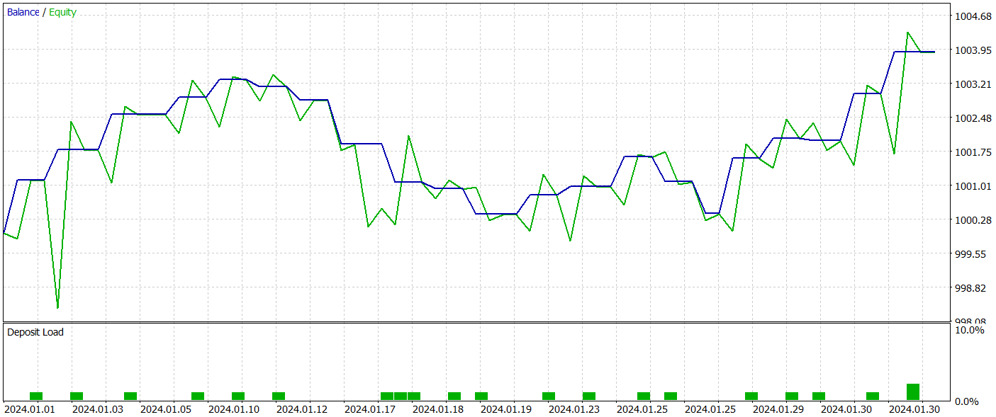
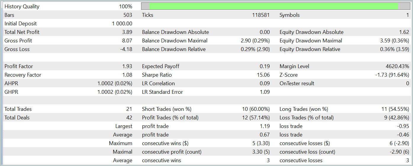
The balance chart during the test period shows an upward trend, which is clearly a positive outcome. However, the model executed only 21 trades during the entire test period, of which 12 were profitable. Unfortunately, this limited number of trades does not allow for a conclusive evaluation of the model's effectiveness over longer periods.

Conclusion

In this article, we discussed with the Mask-Attention-Free Transformer (MAFT) method and its application in algorithmic trading. Unlike traditional Transformer architectures, MAFT offers higher computational efficiency by eliminating the need for data masking and accelerating sequence processing.

The test results confirmed that MAFT can improve prediction accuracy while also reducing model training time.

References

Programs used in the article

#	Name	Type	Description
1	Research.mq5	Expert Advisor	EA for collecting examples
2	ResearchRealORL.mq5	Expert Advisor	EA for collecting examples using the Real-ORL method
3	Study.mq5	Expert Advisor	Model training EA
4	Test.mq5	Expert Advisor	Model testing EA
5	Trajectory.mqh	Class library	System state description structure
6	NeuroNet.mqh	Class library	A library of classes for creating a neural network
7	NeuroNet.cl	Library	OpenCL program code library

Translated from Russian by MetaQuotes Ltd.
Original article: https://www.mql5.com/ru/articles/15973

Attached files |

Download ZIP

MQL5.zip (1878.59 KB)

Warning: All rights to these materials are reserved by MetaQuotes Ltd. Copying or reprinting of these materials in whole or in part is prohibited.