Category Theory in MQL5 (Part 6): Monomorphic Pull-Backs and Epimorphic Push-Outs

Introduction

In our previous article, we discussed how equalizers in category theory can be employed to estimate volatility changes using sampled data. In this follow-up article, we will delve into composition and cones in category theory by exploring the significance of various cone setups on the end results of analysis. We are not looking at another concept of category theory that can be used in forecasting or describing some aspects of the market but rather we are doing a sensitivity analysis of category theory compositions and cones more specifically.

Before we that lets look at the duality of the concept of the last article, co-equalizers.

Co-Equalizers

Coequalizers, the duality of equalizers covered in the previous article are domains that take elements from the codomain that are typically different (recall equalizers focused on the elements that are similar) and through a co-equalizer morphism, produces one element for each domain element disparity. The created common element in the new equalizer domain is done for each element in the domain. This is usually drawn as below:

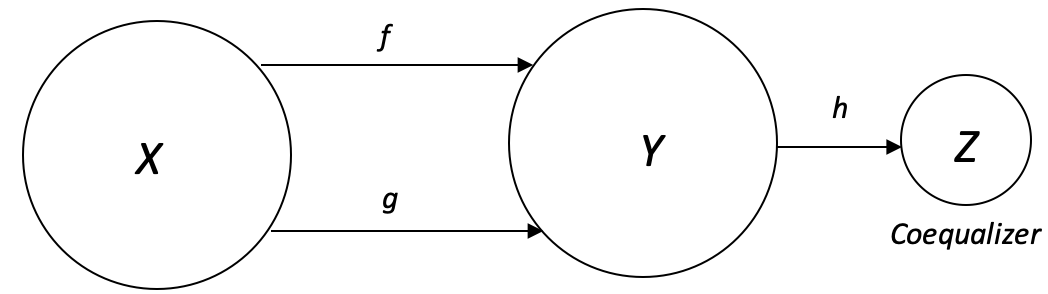
The function h therefore acts as a quotient since for each value d in the domain that may map to different values depending on the morphism (whether f or g) the end result (element) in the coequalizer domain is the same.

An array of values times a ‘common value numerator Z’ divided by the same array of values will always yield the common value. So, the division by the array of values in Y acts like a quotient to Y. This is often represented as:

With h the quotient function defined as 

So, in practice, for traders if we have the following log from recent trading activity;

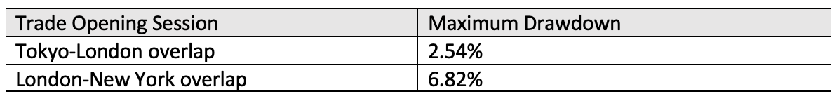
We can infer the following diagram:

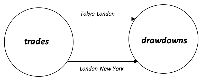
With this diagram we could elect to come up with a co-equalizer that guides our position sizing based on whether we are trading at Tokyo-London overlap or London-New York overlap. If we inversely weight our position sizing based on logged drawdowns we would have a co-equalizer equivalent that is based on a worse case scenario. This can be done without category theory. Where category theory would help would be by applying the universal property. This has already been highlighted in the 2 prior articles. In our case we could compare live drawdown readings to the weighted (worse case) value we weighted our portfolio towards. If the current values are worse than what we were expecting then we would make appropriate changes to our position sizing.

Monomorphic Pull-Backs

A monomorphism is an injective homomorphism that has a domain of a cardinality less than or equal to the codomain with all morphisms from the domain mapping to a distinct element in the codomain. A pull-back in category theory is a domain (aka fiber product) in a cone that, in a typical 4-domain cone, is diagonally opposite the product domain.

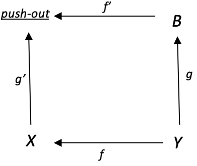
Putting these two concepts together yields an interesting property. If we consider the diagram below:

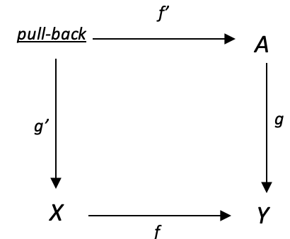
If g: A -->Y is a monomorphism, then for any function f: X -->Y, the left-hand map g’: pull-back --> X in the diagram is also a monomorphism provided there is a commute.

To illustrate this let’s consider a cone with the product domain Y, factor domain X, factor domain A, and the pull-back domain; having EURJPY, EURUSD, USDJPY, and USDX (Dollar-Index) correlation values of the most recent N bars to the prior N bars respectively.

The value of N can be selected from quantile buckets that follow Fibonacci sequence. In our case we will use five values namely 3,5,8,13, and 21. So each domain will have correlations that use each of these periods. These values do change from time to time which is why ontology logs help record all these values for each time. So, an ontology log would therefore have a cone for each period.

We will not use the ontology logs for this article, however we will compute and present tester logs of the values of various cones over a period of 6 months on the weekly timeframe.

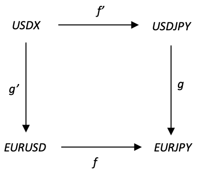
To continue with our diagram above though, the domains each contain correlations across the periods 3,5,8,13, & 21 and the homomorphisms f, g, f’, and g’, will simply pair these across the domains by these periods. So, the correlation between USDX’s 5 most recent weeks and the 5 weeks before that, under f’ will be paired with the correlation USDJPY’s 5 most recent weeks, and the 5 weeks before that, and so on.

The product domain EURJPY will also contain correlation values for the 5 periods mentioned above, however its values will be the result of a product between domain EURUSD and USDJPY. The product from these two will be the geometric mean of the two domains. Now the geometric mean is typically the square root of two products. In our case these products would be the two correlations. Because these correlations can be negative, and we will not delve into imaginary numbers, it is prudent to normalise the correlation value buy having it range from 0.0 to 2.0 as opposed to -1.0 to 1.0. Once the square root/ geometric value has been got, we can then revert to the standard format of -1.0 to 1.0.

So, to normalise we would add 1.0 to the correlation values before computing the geometric mean. Once we have the mean we would simply subtract 1.0 to revert to the standard.

If for control purposes we first run tests with our cone without using the property, but simply using the period length quantile buckets above, from 2021-07-01 to 2022-01-01 (about 26 weeks) on the weekly timeframe, while selecting only the period in USDX with the highest correlation, these will be our results:

2023.04.07 16:05:32.658 ct_6 (USDX-JUN23,W1)                        [,0]               [,1]               [,2]               [,3]               [,4]               [,5]
2023.04.07 16:05:32.658 ct_6 (USDX-JUN23,W1)    [ 0,] " DATE "          ," N period "      ," EURUSD corr. "  ," USDJPY corr. "  ," geometric mean "," actual corr. "  
2023.04.07 16:05:32.658 ct_6 (USDX-JUN23,W1)    [ 1,] "2021.07.04 00:00","13"              ,"0.49"            ,"0.90"            ,"0.69"            ,"0.25"            
2023.04.07 16:05:32.658 ct_6 (USDX-JUN23,W1)    [ 2,] "2021.07.11 00:00","5"               ,"0.70"            ,"0.00"            ,"0.30"            ,"-0.00"           
2023.04.07 16:05:32.658 ct_6 (USDX-JUN23,W1)    [ 3,] "2021.07.18 00:00","5"               ,"0.70"            ,"0.10"            ,"0.37"            ,"0.20"            
2023.04.07 16:05:32.658 ct_6 (USDX-JUN23,W1)    [ 4,] "2021.07.25 00:00","5"               ,"0.50"            ,"-0.20"           ,"0.10"            ,"0.70"            
2023.04.07 16:05:32.658 ct_6 (USDX-JUN23,W1)    [ 5,] "2021.08.01 00:00","5"               ,"0.80"            ,"0.10"            ,"0.41"            ,"0.50"            
2023.04.07 16:05:32.658 ct_6 (USDX-JUN23,W1)    [ 6,] "2021.08.08 00:00","5"               ,"0.80"            ,"0.30"            ,"0.53"            ,"0.20"            
2023.04.07 16:05:32.658 ct_6 (USDX-JUN23,W1)    [ 7,] "2021.08.15 00:00","5"               ,"0.90"            ,"0.30"            ,"0.57"            ,"0.70"            
2023.04.07 16:05:32.658 ct_6 (USDX-JUN23,W1)    [ 8,] "2021.08.22 00:00","5"               ,"0.40"            ,"0.50"            ,"0.45"            ,"0.90"            
2023.04.07 16:05:32.659 ct_6 (USDX-JUN23,W1)    [ 9,] "2021.08.29 00:00","5"               ,"0.20"            ,"0.70"            ,"0.43"            ,"0.50"            
2023.04.07 16:05:32.659 ct_6 (USDX-JUN23,W1)    [10,] "2021.09.05 00:00","5"               ,"-0.20"           ,"0.60"            ,"0.13"            ,"0.00"            
2023.04.07 16:05:32.659 ct_6 (USDX-JUN23,W1)    [11,] "2021.09.12 00:00","21"              ,"0.69"            ,"0.27"            ,"0.46"            ,"-0.79"           
2023.04.07 16:05:32.659 ct_6 (USDX-JUN23,W1)    [12,] "2021.09.19 00:00","5"               ,"0.60"            ,"-0.20"           ,"0.13"            ,"0.50"            
2023.04.07 16:05:32.659 ct_6 (USDX-JUN23,W1)    [13,] "2021.09.26 00:00","5"               ,"0.30"            ,"0.20"            ,"0.25"            ,"0.60"            
2023.04.07 16:05:32.659 ct_6 (USDX-JUN23,W1)    [14,] "2021.10.03 00:00","3"               ,"1.00"            ,"1.00"            ,"1.00"            ,"-0.50"           
2023.04.07 16:05:32.659 ct_6 (USDX-JUN23,W1)    [15,] "2021.10.10 00:00","13"              ,"0.55"            ,"0.49"            ,"0.52"            ,"-0.29"           
2023.04.07 16:05:32.659 ct_6 (USDX-JUN23,W1)    [16,] "2021.10.17 00:00","13"              ,"0.60"            ,"0.65"            ,"0.62"            ,"-0.36"           
2023.04.07 16:05:32.659 ct_6 (USDX-JUN23,W1)    [17,] "2021.10.24 00:00","13"              ,"0.62"            ,"0.51"            ,"0.56"            ,"-0.45"           
2023.04.07 16:05:32.659 ct_6 (USDX-JUN23,W1)    [18,] "2021.10.31 00:00","13"              ,"0.64"            ,"0.53"            ,"0.59"            ,"-0.55"           
2023.04.07 16:05:32.659 ct_6 (USDX-JUN23,W1)    [19,] "2021.11.07 00:00","5"               ,"0.80"            ,"-0.50"           ,"-0.05"           ,"-0.10"           
2023.04.07 16:05:32.659 ct_6 (USDX-JUN23,W1)    [20,] "2021.11.14 00:00","5"               ,"0.50"            ,"0.50"            ,"0.50"            ,"-0.70"           
2023.04.07 16:05:32.659 ct_6 (USDX-JUN23,W1)    [21,] "2021.11.21 00:00","3"               ,"1.00"            ,"1.00"            ,"1.00"            ,"1.00"            
2023.04.07 16:05:32.659 ct_6 (USDX-JUN23,W1)    [22,] "2021.11.28 00:00","3"               ,"0.50"            ,"0.50"            ,"0.50"            ,"1.00"            
2023.04.07 16:05:32.659 ct_6 (USDX-JUN23,W1)    [23,] "2021.12.05 00:00","8"               ,"0.76"            ,"-0.62"           ,"-0.18"           ,"-0.02"           
2023.04.07 16:05:32.659 ct_6 (USDX-JUN23,W1)    [24,] "2021.12.12 00:00","8"               ,"0.62"            ,"-0.52"           ,"-0.12"           ,"-0.12"           
2023.04.07 16:05:32.659 ct_6 (USDX-JUN23,W1)    [25,] "2021.12.19 00:00","8"               ,"0.40"            ,"-0.05"           ,"0.16"            ,"-0.26"           
2023.04.07 16:05:32.659 ct_6 (USDX-JUN23,W1)    [26,] "2021.12.26 00:00","3"               ,"0.50"            ,"0.50"            ,"0.50"            ,"0.50"            

In these results the correlation between geometric mean value and the actual value is -0.07 which implies that our hypothesis of selecting the highest correlation period from USDX does not lead to accurate projections for EURJPY’s values.

If we move on and look at the monomorphism property above, implementation will mean the domains will not have the same cardinality. We had initially chosen a set of periods based on part of Fibonacci series including 3,5,8,13, and 21. From the test run logs above whichever of them had the highest correlation for the dollar index (USDX) was selected. For instance, on 2021-09-05 the period of 5 selection meant the correlation of the current 5 USDX bars to the previous 5, was the highest of all periods 3,5,8,13, & 21, and thus it was chosen and used as the correlation period for EURUSD and USDJPY.

If, however we do apply the monomorphism property to our cone on the parallel sides of say USDJPY à EURJPY and USDX à EURUSD we could get more interesting results. To achieve this, we’ll focus on the cardinality of the domains. Our cone is composed from USDX towards EURJPY and since monomorphism requires an equal or larger codomain when compared to the domain we can easily ensure each homomorphism is injective by increasing domain size from USDX towards EURJPY and avoiding any morphisms mapping to the same element in the codomain.

Our unit for scaling domain size is the quantile buckets of period length we assign to each domain. So, we need to come up with quantile buckets for each domain as we attempted in the prior article. So, putting this together with the flow of our cone implies that domain USDX will have the least buckets but as we progress towards EURJPY the number of quantile buckets per domain will increase.

In order to specifically match our monomorphism property above, we will have |USDX| = 5 as above however we’ll have |EURUSD| = 19, |USDJPY| = 5, and |EURJPY| = 19. So, the periods will not be bucketed according to Fibonacci sequence used above but for domains USDJPY and EURJPY will be used individually within the range 3 to 21. So, the morphisms g and g’, our monomorphisms, will use another indicator to help map from the smaller sized domains, to larger sized domains.

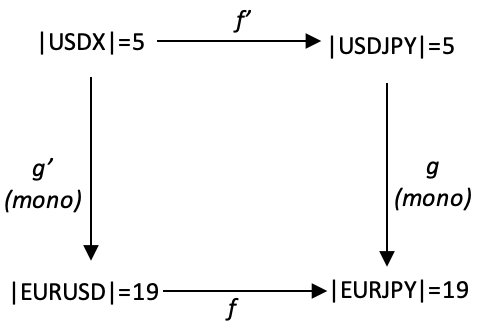
The indicator we’ll use in mapping for morphism g’ and g will be RSI. Since RSI is cyclic and easily normalized from 0-100 it is a fit. You could choose a different similar indicator, but in our case the indicator reading will determine what proportion of the codomain is relevant. The extremes 3, and 21 will remain unchanged as before but a value of 5 will be mapped to either 4,5,6, or 7 in direct proportion to the RSI readings.

Running similar tests as above, using the same period selection criteria within USDX, gives us these logs.

2023.04.07 16:05:32.659 ct_6 (USDX-JUN23,W1)                        [,0]               [,1]               [,2]               [,3]               [,4]               [,5]
2023.04.07 16:05:32.659 ct_6 (USDX-JUN23,W1)    [ 0,] " DATE "          ," N period "      ," EURUSD corr. "  ," USDJPY corr. "  ," geometric mean "," actual corr. "  
2023.04.07 16:05:32.659 ct_6 (USDX-JUN23,W1)    [ 1,] "2021.07.04 00:00","13"              ,"0.13"            ,"0.90"            ,"0.47"            ,"0.24"            
2023.04.07 16:05:32.659 ct_6 (USDX-JUN23,W1)    [ 2,] "2021.07.11 00:00","5"               ,"-0.49"           ,"0.00"            ,"-0.28"           ,"-0.49"           
2023.04.07 16:05:32.659 ct_6 (USDX-JUN23,W1)    [ 3,] "2021.07.18 00:00","5"               ,"0.37"            ,"0.10"            ,"0.23"            ,"-0.09"           
2023.04.07 16:05:32.659 ct_6 (USDX-JUN23,W1)    [ 4,] "2021.07.25 00:00","5"               ,"0.20"            ,"-0.20"           ,"-0.02"           ,"-0.09"           
2023.04.07 16:05:32.659 ct_6 (USDX-JUN23,W1)    [ 5,] "2021.08.01 00:00","5"               ,"0.43"            ,"0.10"            ,"0.25"            ,"0.14"            
2023.04.07 16:05:32.659 ct_6 (USDX-JUN23,W1)    [ 6,] "2021.08.08 00:00","5"               ,"0.26"            ,"0.30"            ,"0.28"            ,"0.37"            
2023.04.07 16:05:32.659 ct_6 (USDX-JUN23,W1)    [ 7,] "2021.08.15 00:00","5"               ,"-0.20"           ,"0.30"            ,"0.02"            ,"0.09"            
2023.04.07 16:05:32.660 ct_6 (USDX-JUN23,W1)    [ 8,] "2021.08.22 00:00","5"               ,"-0.71"           ,"0.50"            ,"-0.35"           ,"0.14"            
2023.04.07 16:05:32.660 ct_6 (USDX-JUN23,W1)    [ 9,] "2021.08.29 00:00","5"               ,"-0.89"           ,"0.70"            ,"-0.56"           ,"-0.31"           
2023.04.07 16:05:32.660 ct_6 (USDX-JUN23,W1)    [10,] "2021.09.05 00:00","5"               ,"-0.77"           ,"0.60"            ,"-0.40"           ,"-0.31"           
2023.04.07 16:05:32.660 ct_6 (USDX-JUN23,W1)    [11,] "2021.09.12 00:00","21"              ,"0.68"            ,"0.27"            ,"0.46"            ,"-0.88"           
2023.04.07 16:05:32.660 ct_6 (USDX-JUN23,W1)    [12,] "2021.09.19 00:00","5"               ,"-0.31"           ,"-0.20"           ,"-0.26"           ,"-0.09"           
2023.04.07 16:05:32.660 ct_6 (USDX-JUN23,W1)    [13,] "2021.09.26 00:00","5"               ,"0.54"            ,"0.20"            ,"0.36"            ,"0.77"            
2023.04.07 16:05:32.660 ct_6 (USDX-JUN23,W1)    [14,] "2021.10.03 00:00","3"               ,"-0.80"           ,"1.00"            ,"-0.37"           ,"-0.20"           
2023.04.07 16:05:32.660 ct_6 (USDX-JUN23,W1)    [15,] "2021.10.10 00:00","13"              ,"0.16"            ,"0.49"            ,"0.32"            ,"-0.42"           
2023.04.07 16:05:32.660 ct_6 (USDX-JUN23,W1)    [16,] "2021.10.17 00:00","13"              ,"0.43"            ,"0.65"            ,"0.53"            ,"-0.47"           
2023.04.07 16:05:32.660 ct_6 (USDX-JUN23,W1)    [17,] "2021.10.24 00:00","13"              ,"0.68"            ,"0.51"            ,"0.59"            ,"-0.53"           
2023.04.07 16:05:32.660 ct_6 (USDX-JUN23,W1)    [18,] "2021.10.31 00:00","13"              ,"0.78"            ,"0.53"            ,"0.65"            ,"-0.58"           
2023.04.07 16:05:32.660 ct_6 (USDX-JUN23,W1)    [19,] "2021.11.07 00:00","5"               ,"0.89"            ,"-0.50"           ,"-0.03"           ,"0.71"            
2023.04.07 16:05:32.660 ct_6 (USDX-JUN23,W1)    [20,] "2021.11.14 00:00","5"               ,"0.89"            ,"0.50"            ,"0.68"            ,"0.37"            
2023.04.07 16:05:32.660 ct_6 (USDX-JUN23,W1)    [21,] "2021.11.21 00:00","3"               ,"-0.40"           ,"1.00"            ,"0.10"            ,"-0.20"           
2023.04.07 16:05:32.660 ct_6 (USDX-JUN23,W1)    [22,] "2021.11.28 00:00","3"               ,"-0.40"           ,"0.50"            ,"-0.05"           ,"1.00"            
2023.04.07 16:05:32.660 ct_6 (USDX-JUN23,W1)    [23,] "2021.12.05 00:00","8"               ,"0.33"            ,"-0.62"           ,"-0.29"           ,"-0.12"           
2023.04.07 16:05:32.660 ct_6 (USDX-JUN23,W1)    [24,] "2021.12.12 00:00","8"               ,"0.43"            ,"-0.52"           ,"-0.17"           ,"-0.23"           
2023.04.07 16:05:32.660 ct_6 (USDX-JUN23,W1)    [25,] "2021.12.19 00:00","8"               ,"0.60"            ,"-0.05"           ,"0.23"            ,"0.10"            
2023.04.07 16:05:32.660 ct_6 (USDX-JUN23,W1)    [26,] "2021.12.26 00:00","3"               ,"0.40"            ,"0.50"            ,"0.45"            ,"-0.80"           

There is no significant statistical difference between the two results sets. And this result -0.08 is none the less incremented by almost 15%. The cone and linkage of the domains, with their various elements (in this case correlation) does certainly present an opportunity in studying for patterns and trends that could not be conspicuous per se and yet are very definitive in trading.

Epimorphic Push-Outs

An epimorphism is a surjective homomorphism that has its domain with a larger cardinal than the codomain and with morphisms from the domain mapping to all elements in the codomain meaning none are left unlinked. A push-out in category theory is a domain (aka fiber coproduct) in a cone that, in a typical 4-domain cone, is diagonally opposite the coproduct domain.

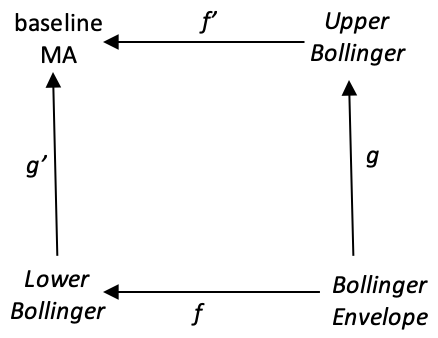
Putting these two together as we did with the monomorphic pullbacks, also gives us a property. This is shown in the diagram below:

If g: Y à B is an epimorphism, then for any function f: Y --> X, the left-hand map g’: X --> push-out in the diagram is also an epimorphism. To explore this let’s again consider a cone with the coproduct domain Y being Bollinger Envelope range values for any security’s bid prices. The two coproduct factor domains (X and B) will be the Bollinger bands upper envelope and the lower envelope. The difference (or ‘coproduct union’) between these two will provide our forecast for the Bollinger Envelope range. The pushout domain will be the baseline moving average of Bollinger bands from which the upper and lower envelopes are derived.

Just like we used period lengths as a variable for coming up with various correlation coefficients in the monomorphic pullbacks above, we will again use period lengths for deriving various moving average values for each domain that give us a wide variety of Bollinger envelopes. For our exploratory test, as above, we can begin with the periods 3,5,8,13, and 21.

So, our cone is composed from the Bollinger Envelope domain towards the Baseline MA domain. It is composed in a direction opposite to our first cone on monomorphic push-outs because its apex is a coproduct and not a product as before. The morphisms arrows show homomorphism direction. The linking of the elements in each domain will simply follow respective N period as we had above.

So, if we run a test, before applying the epimorphic property, by selecting periods at the baseline-MA domain based on minimum standard deviation we will have these logs:

2023.04.07 19:04:11.241 ct_6 (USDX-JUN23,W1)                        [,0]               [,1]               [,2]               [,3]               [,4]               [,5]               [,6]
2023.04.07 19:04:11.241 ct_6 (USDX-JUN23,W1)    [ 0,] " DATE "          ," N period "      ," Baseline-MA "   ," Upper Bands "   ," Lower Bands "   ," Envelope Delta "," Actual Range "  
2023.04.07 19:04:11.241 ct_6 (USDX-JUN23,W1)    [ 1,] "2021.07.04 00:00","8"               ,"103.425"         ,"105.548"         ,"101.301"         ,"4.248"           ,"0.850"           
2023.04.07 19:04:11.241 ct_6 (USDX-JUN23,W1)    [ 2,] "2021.07.11 00:00","8"               ,"103.425"         ,"105.548"         ,"101.301"         ,"4.248"           ,"0.758"           
2023.04.07 19:04:11.241 ct_6 (USDX-JUN23,W1)    [ 3,] "2021.07.18 00:00","13"              ,"102.993"         ,"105.163"         ,"100.822"         ,"4.341"           ,"0.691"           
2023.04.07 19:04:11.241 ct_6 (USDX-JUN23,W1)    [ 4,] "2021.07.25 00:00","13"              ,"102.993"         ,"105.163"         ,"100.822"         ,"4.341"           ,"1.193"           
2023.04.07 19:04:11.241 ct_6 (USDX-JUN23,W1)    [ 5,] "2021.08.01 00:00","13"              ,"102.993"         ,"105.163"         ,"100.822"         ,"4.341"           ,"1.030"           
2023.04.07 19:04:11.241 ct_6 (USDX-JUN23,W1)    [ 6,] "2021.08.08 00:00","13"              ,"102.993"         ,"105.163"         ,"100.822"         ,"4.341"           ,"0.735"           
2023.04.07 19:04:11.241 ct_6 (USDX-JUN23,W1)    [ 7,] "2021.08.15 00:00","21"              ,"103.616"         ,"106.326"         ,"100.906"         ,"5.420"           ,"1.270"           
2023.04.07 19:04:11.241 ct_6 (USDX-JUN23,W1)    [ 8,] "2021.08.22 00:00","21"              ,"103.616"         ,"106.326"         ,"100.906"         ,"5.420"           ,"0.868"           
2023.04.07 19:04:11.241 ct_6 (USDX-JUN23,W1)    [ 9,] "2021.08.29 00:00","21"              ,"103.616"         ,"106.326"         ,"100.906"         ,"5.420"           ,"0.854"           
2023.04.07 19:04:11.241 ct_6 (USDX-JUN23,W1)    [10,] "2021.09.05 00:00","21"              ,"103.616"         ,"106.326"         ,"100.906"         ,"5.420"           ,"0.750"           
2023.04.07 19:04:11.241 ct_6 (USDX-JUN23,W1)    [11,] "2021.09.12 00:00","21"              ,"103.616"         ,"106.326"         ,"100.906"         ,"5.420"           ,"0.912"           
2023.04.07 19:04:11.241 ct_6 (USDX-JUN23,W1)    [12,] "2021.09.19 00:00","21"              ,"103.616"         ,"106.326"         ,"100.906"         ,"5.420"           ,"0.565"           
2023.04.07 19:04:11.241 ct_6 (USDX-JUN23,W1)    [13,] "2021.09.26 00:00","21"              ,"103.616"         ,"106.326"         ,"100.906"         ,"5.420"           ,"1.325"           
2023.04.07 19:04:11.241 ct_6 (USDX-JUN23,W1)    [14,] "2021.10.03 00:00","21"              ,"103.616"         ,"106.326"         ,"100.906"         ,"5.420"           ,"0.770"           
2023.04.07 19:04:11.241 ct_6 (USDX-JUN23,W1)    [15,] "2021.10.10 00:00","21"              ,"103.616"         ,"106.326"         ,"100.906"         ,"5.420"           ,"0.811"           
2023.04.07 19:04:11.241 ct_6 (USDX-JUN23,W1)    [16,] "2021.10.17 00:00","21"              ,"103.616"         ,"106.326"         ,"100.906"         ,"5.420"           ,"0.700"           
2023.04.07 19:04:11.241 ct_6 (USDX-JUN23,W1)    [17,] "2021.10.24 00:00","21"              ,"103.616"         ,"106.326"         ,"100.906"         ,"5.420"           ,"1.035"           
2023.04.07 19:04:11.241 ct_6 (USDX-JUN23,W1)    [18,] "2021.10.31 00:00","21"              ,"103.616"         ,"106.326"         ,"100.906"         ,"5.420"           ,"0.842"           
2023.04.07 19:04:11.241 ct_6 (USDX-JUN23,W1)    [19,] "2021.11.07 00:00","21"              ,"103.616"         ,"106.326"         ,"100.906"         ,"5.420"           ,"1.400"           
2023.04.07 19:04:11.241 ct_6 (USDX-JUN23,W1)    [20,] "2021.11.14 00:00","13"              ,"102.993"         ,"105.163"         ,"100.822"         ,"4.341"           ,"1.305"           
2023.04.07 19:04:11.241 ct_6 (USDX-JUN23,W1)    [21,] "2021.11.21 00:00","13"              ,"102.993"         ,"105.163"         ,"100.822"         ,"4.341"           ,"0.933"           
2023.04.07 19:04:11.241 ct_6 (USDX-JUN23,W1)    [22,] "2021.11.28 00:00","21"              ,"103.616"         ,"106.326"         ,"100.906"         ,"5.420"           ,"1.115"           
2023.04.07 19:04:11.241 ct_6 (USDX-JUN23,W1)    [23,] "2021.12.05 00:00","21"              ,"103.616"         ,"106.326"         ,"100.906"         ,"5.420"           ,"0.747"           
2023.04.07 19:04:11.241 ct_6 (USDX-JUN23,W1)    [24,] "2021.12.12 00:00","21"              ,"103.616"         ,"106.326"         ,"100.906"         ,"5.420"           ,"1.077"           
2023.04.07 19:04:11.242 ct_6 (USDX-JUN23,W1)    [25,] "2021.12.19 00:00","21"              ,"103.616"         ,"106.326"         ,"100.906"         ,"5.420"           ,"0.685"           
2023.04.07 19:04:11.242 ct_6 (USDX-JUN23,W1)    [26,] "2021.12.26 00:00","21"              ,"103.616"         ,"106.326"         ,"100.906"         ,"5.420"           ,"0.778"           

Our correlation check between the analysis and actual stands at 0.12 which is still not significant.

This brings us to the epimorphism property. If we do apply it to our cone on the parallel sides of say LOWER-BOLLINGER --> BASELINE-MA and BOLLINGER-ENVELOPE --> UPPER-BOLLINGER we could potentially get different results. To achieve this, we’ll focus once again on the cardinality of the domains. Our cone is composed towards BASELINE-MA from BOLLINGER-ENVELOPE given that it’s a coproduct and not a product as prior. Since epimorphisms require an equal or larger domain when compared to the codomain we can easily ensure each homomorphism is surjective by increasing codomain size from BOLLINGER-ENVELOPE towards BASELINE-MA and also seeing to it that all elements in each respective codomain are mapped to.

As was the case above, since we had applied a Fibonacci based quantile bucketing we can simply be explicit on the domains we would like to be larger. This as above implies our cardinals will be | LOWER-BOLLINGER| = 19 and also | BOLLINGER-ENVELOPE | = 19. The larger domains remain at the apex and lower factor domain because the composition is reversed given the coproduct.

Test runs with these settings give us the results below:

2023.04.07 19:58:57.547 ct_6 (USDX-JUN23,W1)                        [,0]               [,1]               [,2]               [,3]               [,4]               [,5]               [,6]
2023.04.07 19:58:57.547 ct_6 (USDX-JUN23,W1)    [ 0,] " DATE "          ," N period "      ," Baseline-MA "   ," Upper Bands "   ," Lower Bands "   ," Envelope Delta "," Actual Range "  
2023.04.07 19:58:57.547 ct_6 (USDX-JUN23,W1)    [ 1,] "2021.07.04 00:00","8"               ,"103.425"         ,"105.548"         ,"101.301"         ,"4.248"           ,"0.850"           
2023.04.07 19:58:57.547 ct_6 (USDX-JUN23,W1)    [ 2,] "2021.07.11 00:00","8"               ,"103.425"         ,"105.548"         ,"101.301"         ,"4.248"           ,"0.758"           
2023.04.07 19:58:57.547 ct_6 (USDX-JUN23,W1)    [ 3,] "2021.07.18 00:00","13"              ,"102.993"         ,"105.163"         ,"100.822"         ,"4.341"           ,"0.691"           
2023.04.07 19:58:57.547 ct_6 (USDX-JUN23,W1)    [ 4,] "2021.07.25 00:00","13"              ,"102.993"         ,"105.163"         ,"100.822"         ,"4.341"           ,"1.193"           
2023.04.07 19:58:57.547 ct_6 (USDX-JUN23,W1)    [ 5,] "2021.08.01 00:00","13"              ,"102.993"         ,"105.163"         ,"100.822"         ,"4.341"           ,"1.030"           
2023.04.07 19:58:57.547 ct_6 (USDX-JUN23,W1)    [ 6,] "2021.08.08 00:00","13"              ,"102.993"         ,"105.163"         ,"100.822"         ,"4.341"           ,"0.735"           
2023.04.07 19:58:57.547 ct_6 (USDX-JUN23,W1)    [ 7,] "2021.08.15 00:00","21"              ,"103.616"         ,"106.326"         ,"100.906"         ,"5.420"           ,"1.270"           
2023.04.07 19:58:57.547 ct_6 (USDX-JUN23,W1)    [ 8,] "2021.08.22 00:00","21"              ,"103.616"         ,"106.326"         ,"100.906"         ,"5.420"           ,"0.868"           
2023.04.07 19:58:57.547 ct_6 (USDX-JUN23,W1)    [ 9,] "2021.08.29 00:00","21"              ,"103.616"         ,"106.326"         ,"100.906"         ,"5.420"           ,"0.854"           
2023.04.07 19:58:57.547 ct_6 (USDX-JUN23,W1)    [10,] "2021.09.05 00:00","21"              ,"103.616"         ,"106.326"         ,"100.906"         ,"5.420"           ,"0.750"           
2023.04.07 19:58:57.547 ct_6 (USDX-JUN23,W1)    [11,] "2021.09.12 00:00","21"              ,"103.616"         ,"106.326"         ,"100.906"         ,"5.420"           ,"0.912"           
2023.04.07 19:58:57.547 ct_6 (USDX-JUN23,W1)    [12,] "2021.09.19 00:00","21"              ,"103.616"         ,"106.326"         ,"100.906"         ,"5.420"           ,"0.565"           
2023.04.07 19:58:57.547 ct_6 (USDX-JUN23,W1)    [13,] "2021.09.26 00:00","21"              ,"103.616"         ,"106.326"         ,"100.906"         ,"5.420"           ,"1.325"           
2023.04.07 19:58:57.547 ct_6 (USDX-JUN23,W1)    [14,] "2021.10.03 00:00","21"              ,"103.616"         ,"106.326"         ,"100.906"         ,"5.420"           ,"0.770"           
2023.04.07 19:58:57.548 ct_6 (USDX-JUN23,W1)    [15,] "2021.10.10 00:00","21"              ,"103.616"         ,"106.326"         ,"100.906"         ,"5.420"           ,"0.811"           
2023.04.07 19:58:57.548 ct_6 (USDX-JUN23,W1)    [16,] "2021.10.17 00:00","21"              ,"103.616"         ,"106.326"         ,"100.906"         ,"5.420"           ,"0.700"           
2023.04.07 19:58:57.548 ct_6 (USDX-JUN23,W1)    [17,] "2021.10.24 00:00","21"              ,"103.616"         ,"106.326"         ,"100.906"         ,"5.420"           ,"1.035"           
2023.04.07 19:58:57.548 ct_6 (USDX-JUN23,W1)    [18,] "2021.10.31 00:00","21"              ,"103.616"         ,"106.326"         ,"100.906"         ,"5.420"           ,"0.842"           
2023.04.07 19:58:57.548 ct_6 (USDX-JUN23,W1)    [19,] "2021.11.07 00:00","21"              ,"103.616"         ,"106.326"         ,"100.906"         ,"5.420"           ,"1.400"           
2023.04.07 19:58:57.548 ct_6 (USDX-JUN23,W1)    [20,] "2021.11.14 00:00","13"              ,"102.993"         ,"105.163"         ,"100.822"         ,"4.341"           ,"1.305"           
2023.04.07 19:58:57.548 ct_6 (USDX-JUN23,W1)    [21,] "2021.11.21 00:00","13"              ,"102.993"         ,"105.163"         ,"100.822"         ,"4.341"           ,"0.933"           
2023.04.07 19:58:57.548 ct_6 (USDX-JUN23,W1)    [22,] "2021.11.28 00:00","21"              ,"103.616"         ,"106.326"         ,"100.906"         ,"5.420"           ,"1.115"           
2023.04.07 19:58:57.548 ct_6 (USDX-JUN23,W1)    [23,] "2021.12.05 00:00","21"              ,"103.616"         ,"106.326"         ,"100.906"         ,"5.420"           ,"0.747"           
2023.04.07 19:58:57.548 ct_6 (USDX-JUN23,W1)    [24,] "2021.12.12 00:00","21"              ,"103.616"         ,"106.326"         ,"100.906"         ,"5.420"           ,"1.077"           
2023.04.07 19:58:57.548 ct_6 (USDX-JUN23,W1)    [25,] "2021.12.19 00:00","21"              ,"103.616"         ,"106.326"         ,"100.906"         ,"5.420"           ,"0.685"           
2023.04.07 19:58:57.548 ct_6 (USDX-JUN23,W1)    [26,] "2021.12.26 00:00","21"              ,"103.616"         ,"106.326"         ,"100.906"         ,"5.420"           ,"0.778"           

Again, the results differ to 0.16, which represents a change of more than 30%.

Conclusion

In conclusion we have looked at how the cone compositions of its domains can be linked and analyzed in ways that are not always evident by looking at indicators and time series. Cone’s in category theory present a lot of permutations in pairing domains that in itself leads to multiple ways of looking at, interpreting, and therefore making projections. Specifically, in this article we’ve seen how making slight restrictive adjustments to cone composition by applying monomorphic pull-backs and epimorphic push-outs, can change end results by 15 - 30%. Looking at the morphisms by applying weighting and other changes one can not only develop novel entry signals, but also adept money management systems. With our script file attached to this article, the reader may fine tune this to his particular indicators and trading style.