MQL5 Wizard Techniques you should know (Part 18): Neural Architecture Search with Eigen Vectors

Preface

We continue the series on MQL5 wizard implementation by looking into Neural Architecture Search while specifically dwelling on the role Eigen Vectors can play in making this process, of expediting network training, more efficient. Neural networks are arguably the fitting of a curve to a set of data in that they help come up with a formulaic expression that, when applied to input data (x), provides a target value (y) just like a quadratic equation does with a curve. The x and y data points though can be, and in fact are often, multidimensional, which is why neural networks have gained a lot of popularity. Nonetheless, the principle of coming up with a formulaic expression does remain, which is why neural networks are simply a means of arriving at this but not the only way of doing so.

Introduction

If we choose to use neural networks to define the relationship between a training dataset and its target, as is the case for this article, then we have to contend with the question of what settings will this network use? There are several types of networks, and this implies the applicable designs and settings are also many. For this article, we consider a very basic case that is often referred to as a multi-layer perceptron. With this type, the settings we’ll dwell on will be only the number of hidden layers and the size of each hidden layer.

NAS can typically help identify these 2 settings and much more. For instance, even with simple MLPs the question of which activation type to use, the initial weights to use, as well as the initial biases are all factors that are sensitive to the performance and accuracy of the network. These though are skimmed over here because the search space is very extensive and the compute resources required for forward and back propagation on even a moderate sized data set would be prohibitive.

The approach at NAS to be adopted here though is a bit novel in that it engages eigen vectors & values in a matrix search space to identify the ideal settings. Conventionally NAS is carried out either via reinforcement learning, or evolutionary algorithms, or Bayesian optimization, or random search.

Each of these conventional approaches involves training and cross validating a network with its selected settings (aka architecture) by benchmarking each performance from the target, for comparison purposes. What sets them apart is how exhaustive they are, or their approach at being efficient without being exhaustive within the search space. Reinforcement learning relies on an algorithm that pre-evaluates a network within the search space based on its settings, and it keeps improving this algorithm with each selection. Evolutionary algorithms cross or combine networks within the search space to arrive at new networks that may not have necessarily been in the search space to begin with, again by evaluating their performance benchmarked of a target. Bayesian optimization like random search relies on the search space being sorted in an array format or where the different network settings can be perceived as co-ordinates within the search space. For example, if a search space is 2-dimensional with only 2 variables the standard size of a hidden layer, and the number of hidden layers then these options would be spread out across this matrix in an ascending (or descending) order across its diagonal in a format similar to the below image.

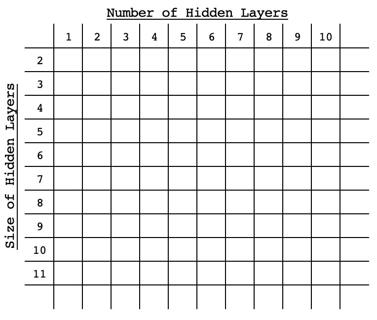
With this arrangement the performance of any network would be pegged to its ‘coordinates’ within the space, thus statistical methods would be used with each subsequent selection to refine the choice of network that would yield the best performance. This article on eigen vectors and PCA that was written a few days back used a matrix search space to select an ideal weekday and indicator applied price, to trade the EURUSD when using the 4-hour timeframe. This was from a cross matrix of price changes for each of the 5-week days and in each of the considered applied prices.

We will consider a similar search approach for this article. Since exhaustive training of all networks is a problem we are trying to ‘solve’, our benchmarks will simply be forward pass scores from the target values on networks that are initialized with standard weights and biases. We’ll make only forward runs on a data sample, and the mean score for each setting will serve as its benchmark within the matrix.

The Role of Eigenvectors in NAS

The eigen matrix we’ll use for NAS will be 2-dimensional for brevity, as alluded to above. If we consider a simple MLP where all hidden layers have the same size, the only 2 questions we’ll want answered will be how many hidden layers should the MLP have and what size is each hidden layer.

The possible answers to these questions can easily be presented in a matrix, with the default performance of each network logged at each layer-size and layer-number combination. The networks will vary in settings as reflected in the matrix table, however their input and output layers will be standard. For this article, we will have an input layer of size 4, and an output layer of size 1. We are looking at an ordinary scenario where we forecast the next close price based on the 4 last close price values.

The test symbol will be EURJPY over the year 2022 on the 4-hr time frame. This means our data will be 4-hour close prices for the year 2022. In ‘training’ this model, all we’re doing is logging the mean deviance from the target values throughout the year for all network settings. Our settings will span from single hidden layer up to 10 hidden layers along the matrix rows, while the columns will feature the hidden layer sizes, which will span from 2 to 11. These test settings are arbitrary and since complete source code is attached at the end of this article, the reader is welcome to customize it to his preference.

To reiterate, the ‘training’ of the model will involve a single forward pass of each of the available networks, all with the standard default weights and biases over the year 2022 with each bar forecast benchmarked against the actual close price. There will be no back-propagation or typical network training during this ‘training’.

We rely on a network class we looked at in this article to implement the MLP. It simply requires an integer array whose size defines the total number of layers, where the integer value at each index sets the layer size.

Even though this article and series are highlighting the MQL5 wizard, the ‘training’ mentioned above will be done by script as was the case in the last eigen vectors article, and we’ll use the results/ recommendations from it to code a signal class instance for testing with a wizard assembled expert advisor. Our testing of the assembled expert advisor will have the usual network training on each bar or with each new data point. The strategy tester result of the recommended network will be benchmarked against the worst recommendation, as a control, so we can evaluate the thesis whether eigen vectors and values can be resourceful in NAS.

If we do a recap of what we covered in the last article on eigen vectors and values, though, the dimensionality reduction used provided us with a single vector from a matrix under analysis. So, in our case, the logged performance of each network that we have in a matrix will be reduced to a vector. In the last article, we wanted to get the weekday and applied price that captured most of the variance of the pair EURJPY over a year on the 4-hr time frame. This implied we focused on the maximum values of the eigen vectors within the projected matrix, since they positively correlated the most with our target.

In this case, though, our matrix has logged deviations from target values, implying what we have in our matrix is the error factor of each network. Since for testing purposes we want to use the network with the least error, our selections for network by number of layers and size of each layer will be the minimums in each of the eigen vectors as retrieved from the projection matrix. This pre-processing as mentioned is all handled by script, and it can be divided into 5 sections, namely the a) initialization of the networks:

//initialise networks
   ArrayResize(__M.row, __SIZE);
   for(int r = 0; r < __SIZE; r++)
   {  for(int c = 0; c < __SIZE; c++)
      {  ArrayResize(__M.row[r].col, __SIZE);
         ArrayResize(__M.row[r].col[c].settings, 2 + __LEAST_LAYERS + r);
         ArrayFill(__M.row[r].col[c].settings, 0, __LEAST_LAYERS + r + 2, __LEAST_SIZE + c);
         __M.row[r].col[c].settings[0] = __INPUTS;
         __M.row[r].col[c].settings[__LEAST_LAYERS + r + 1] = __OUTPUTS;
         __M.row[r].col[c].n = new Cnetwork(__M.row[r].col[c].settings, __initial_weight, __initial_bias);
      }
   }

b) benchmarking of the networks:

//benchmark networks
   int _buffer_size = (52*PeriodSeconds(PERIOD_W1))/PeriodSeconds(Period());
   PrintFormat(__FUNCSIG__ + " buffered: %i", _buffer_size);
   if(_buffer_size >= __INPUTS)
   {  for(int i = _buffer_size - 1; i >= 0; i--)
      {  for(int r = 0; r < __SIZE; r++)
         {  for(int c = 0; c < __SIZE; c++)
            {  vector _in,_out;
               vector _in_new,_out_new,_in_old,_out_old;
               _in_new.CopyRates(Symbol(), Period(), 8, i + 1, __INPUTS);
               _in_old.CopyRates(Symbol(), Period(), 8, i + 1 + 1, __INPUTS);
               _out_new.CopyRates(Symbol(), Period(), 8, i, __OUTPUTS);
               _out_old.CopyRates(Symbol(), Period(), 8, i + 1, __OUTPUTS);
               _in = Norm(_in_new, _in_old);
               _out = Norm(_out_new, _out_old);
               __M.row[r].col[c].n.Set(_in);
               __M.row[r].col[c].n.Forward();
               __M.row[r].col[c].benchmark += fabs(__M.row[r].col[c].n.output[0]-_out[0]);
            }
         }
      }
   }

c) copying benchmarks to analysis matrix:

//copy benchmarks to analysis matrix
   matrix _m;
   _m.Init(__SIZE, __SIZE);
   _m.Fill(0.0);
   for(int r = 0; r < __SIZE; r++)
   {  for(int c = 0; c < __SIZE; c++)
      {  _m[r][c] = __M.row[r].col[c].benchmark;
      }
   }

d) normalizing the matrix and generating the eigen vectors and values:

//generating eigens
   PrintFormat(" for: %s, with: %s", Symbol(), EnumToString(Period()));
   matrix _z = ZNorm(_m);
   matrix _cov_col = _z.Cov(false);
   matrix _e_vectors;
   vector _e_values;
   _cov_col.Eig(_e_vectors, _e_values);

e) and finally interpreting the eigen vectors to retrieve ideal and worst network layer numbers and layer sizes from the projection matrix:

//interpreting the eigens from projection
   matrix _t = _e_vectors.Transpose();
   matrix _p = _m * _t;
   vector _max_row = _p.Max(0);
   vector _max_col = _p.Max(1);
   string _layers[__SIZE];
   for(int i=0;i<__SIZE;i++)
   {  _layers[i] = IntegerToString(i + __LEAST_LAYERS)+" layer";
   }
   double _nr_layers[];
   _max_row.Swap(_nr_layers);
   //since network performance inversely relates to network deviation from target
   PrintFormat(" est. ideal nr. of layers is: %s", _layers[ArrayMinimum(_nr_layers)]);
   PrintFormat(" est. worst nr. of layers is: %s", _layers[ArrayMaximum(_nr_layers)]);
   string _sizes[__SIZE];
   for(int i=0;i<__SIZE;i++)
   {  _sizes[i] = "size "+IntegerToString(i + __LEAST_SIZE);
   }
   double _size_nr[];
   _max_col.Swap(_size_nr);
   PrintFormat(" est. ideal size of layers is: %s", _sizes[ArrayMinimum(_size_nr)]);
   PrintFormat(" est. worst size of layers is: %s", _sizes[ArrayMaximum(_size_nr)]);

The execution of the above script in a search space of 100 runs for a few seconds, which is a good sign. However, one could argue the space is not comprehensive enough and that is a valid argument, which is why the attached script has the size attributes of the space as a global variable which the user can modify to create something more diligent. In addition, we needed a struct to handle network instances and their benchmarks. This is defined in the header as follows:

//+------------------------------------------------------------------+
//|                                                                  |
//+------------------------------------------------------------------+
struct Scol
{  int   settings[];
   Cnetwork *n;
   double benchmark;
   
   Scol()
   {  ArrayFree(settings);
      benchmark = 0.0;
   }
   ~Scol(){ delete n; };
};
struct Srow
{  Scol  col[];

   Srow(){};
   ~Srow(){};
};
struct Smatrix
{  Srow  row[];
   
   Smatrix(){};
   ~Smatrix(){};
};
Smatrix __M;   //matrix of networks

Testing the Expert Advisor

If we run the above script that helps screen for ideal network settings, we get the following logs, when attached to EURJPY on the 4-hr time frame:

2024.05.03 18:22:39.336 nas_1_changes (EURJPY.ln,H4) void OnStart() buffered: 2184

2024.05.03 18:22:42.209 nas_1_changes (EURJPY.ln,H4) for: EURJPY.ln, with: PERIOD_H4

2024.05.03 18:22:42.209 nas_1_changes (EURJPY.ln,H4) est. ideal nr. of layers is: 6 layer

2024.05.03 18:22:42.209 nas_1_changes (EURJPY.ln,H4) est. worst nr. of layers is: 9 layer

2024.05.03 18:22:42.209 nas_1_changes (EURJPY.ln,H4) est. ideal size of layers is: size 2

2024.05.03 18:22:42.209 nas_1_changes (EURJPY.ln,H4) est. worst size of layers is: size 4

The recommended network settings are for a 6-layer network, where the size of each is 2! As a side note, the target data (y values) used to benchmark the matrix were normalized to be in the range 0.0 to 1.0 where a 0.5 reading implies the resulting price change was 0 while any value less than 0.5 would indicate a resulting price drop and a value above 0.5 would point to a rise in price. The code to the function that does this normalization is listed below:

//+------------------------------------------------------------------+
//| Normalization (0.0 - 1.0, with 0.5 for 0                         |
//+------------------------------------------------------------------+
vector Norm(vector &A, vector &B)
{  vector _n;
   _n.Init(A.Size());
   if(A.Size() > 0 && B.Size() > 0 && A.Size() == B.Size() && A.Min() > 0.0 && B.Min() > 0.0)
   {  int _size = int(A.Size());
      _n.Fill(0.5);
      for(int i = 0; i < _size; i++)
      {  if(A[i] > B[i])
         {  _n[i] += (0.5*((A[i] - B[i])/A[i]));
         }
         else if(A[i] < B[i])
         {  _n[i] -= (0.5*((B[i] - A[i])/B[i]));
         }
      }
   }
   return(_n);
}

This normalization was necessary because given the small data set we are considering training a network to develop weights and biases capable of handling negative and positive values as outputs would require extensively large data sets, more complex network settings and certainly more compute resources. Neither of these scenarios are explored in this article but can be ventured into if deemed feasible. So, with our normalization, we are able to get sensitive results from our network with modest training and data sets.

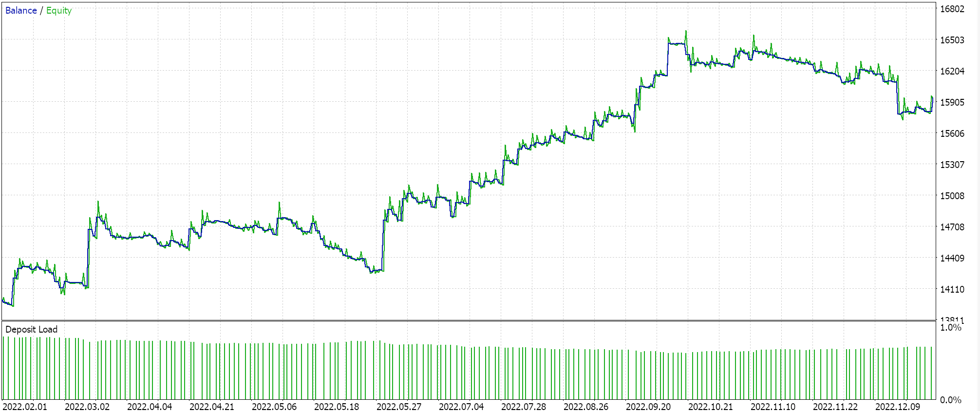
If we run tests with the recommended network configuration of 6 layers at a size of 2 we do get the report and equity curve presented below:

Also flagged in the script log results was the network configuration of 9 layers, sized at 4. If we run tests with identical expert input settings for this network configuration, we get the following results:

Shockingly, the results are almost identical! Why!? Well, there are a few theoretical reasons that could explain this:

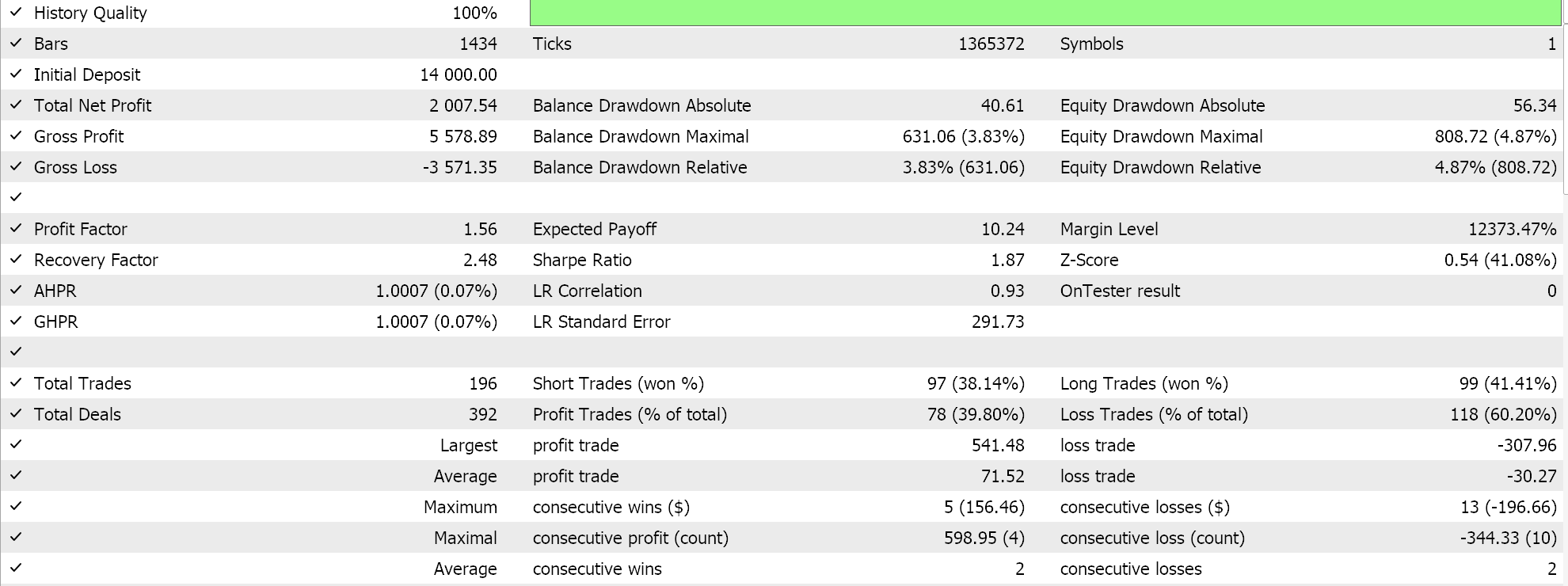
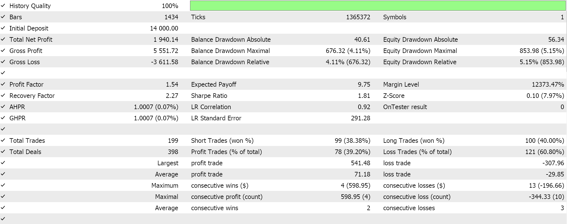
Neural Networks can suffer from redundancy in their capacity, where different settings (or architectures) learn the same underlying relationships in the data even though they have different structures. Recall, in both passes the networks were training so both weights and biases were getting improved. So, while Eigen vectors with the more variance capture a broader set of features and those with the lesser variance focus on details, either network configuration can learn the basics for good performance.

While the number of hidden layers and their size are crucial factors in determining network performance in this situation, there could be other dominant factors at play, like our choice of activation function (we use soft plus) or the used learning rate. Each or all of these could have had a disproportionate influence on the networks’ performance.

Another possible explanation could be to do with search space limitations. We considered 10 different layer sizes and 10 different hidden layer options, all morphing to a rectangular form. This inherently could have restricted the possible network combinations when mapping this particular data set such that either one of these few options could easily arrive at the desired solution.

Conclusion

We have seen how NAS can be done unorthodoxly with eigen vectors and values when faced with a modest scope of neural network configurations to choose from. This process can be scaled and perhaps even expanded to include or consider other factors that were not part of the analysis matrix by adding hidden layer form (we looked only at rectangles) or even activation types. The latter is easiest to add to a matrix like the one looked at in this article since there are only 2 – 3 main types of activation and this could simply mean tripling the number of columns while also expanding the number of rows to ensure a square matrix is maintained, a prerequisite for eigen vector analysis. The addition of hidden layer form could also be done similarly if the various forms that are to be considered are enumerated in clear types. 

Notes:

Attached files can be used by following guides on Expert Advisor Wizard assembly that are found here and here.